class: center, middle, title-slide count: false # Part 3: Convolutional layers. Siamese Networks .bold[Andrei Bursuc ] <br/> .width-10[] url: https://abursuc.github.io//slides/polytechnique/03_cnns_siamese.html .citation[ With slides from A. Karpathy, F. Fleuret, J. Johnson, S. Yeung, G. Louppe, Y. Avrithis ...] --- # Previously ## Neural networks ## Backpropagation --- # The neuron Inspired by neuroscience and human brain, but resemblances do not go too far .center[<img src="images/part3/neuron_2.png" style="height: 350px;"/>] .credit[Slide credit: A. Karpathy] --- # Multi-layer perceptron Layers can be composed *in series*, such that: $$\begin{aligned} \mathbf{h}\_0 &= \mathbf{x} \\\\ \mathbf{h}\_1 &= \sigma(\mathbf{W}\_1^T \mathbf{h}\_0 + \mathbf{b}\_1) \\\\ ... \\\\ \mathbf{h}\_L &= \sigma(\mathbf{W}\_L^T \mathbf{h}\_{L-1} + \mathbf{b}\_L) \\\\ f(\mathbf{x}; \theta) &= \mathbf{h}\_L \end{aligned}$$ where $\theta$ denotes the model parameters $\\{ \mathbf{W}\_k, \mathbf{b}\_k, ... | k=1, ..., L\\}$. - This model is the **multi-layer perceptron**, also known as the _fully connected feedforward network_. - Optionally, the last activation $\sigma$ can be skipped to produce unbounded output values $\hat{y} \in \mathbb{R}$. --- class: center, middle <!-- # Computational graph view --> .width-100[<img src="images/part3/mlp.png" >] <!-- .caption[Computational graph view] --> ## Computational graph view .credit[Figure credit: G. Louppe] --- class: center, middle .center.width-70[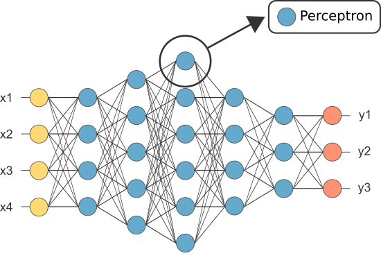] ## More canonical view (with units and connections) --- class: center, middle .center.width-70[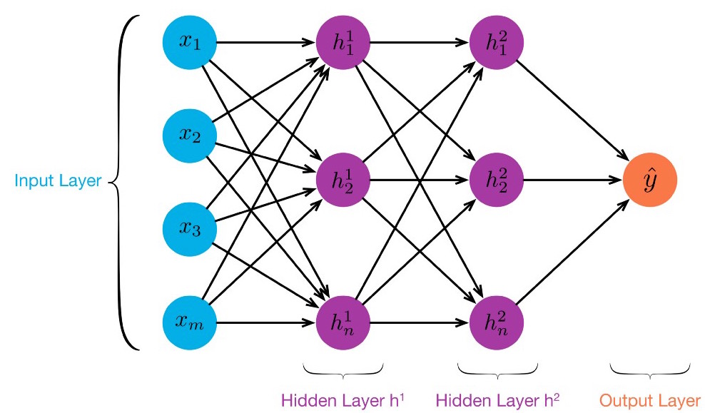] ## More canonical view (with units and connections) --- # Element-wise activation functions - Each neuron/unit is followed by a dedicated activation function - Historically the _sigmoid_ and _tanh_ have been the most popular .center.width-50[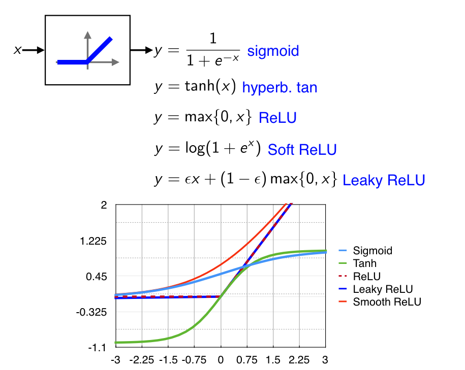] - [Many other activation functions available](https://dashee87.github.io/data%20science/deep%20learning/visualising-activation-functions-in-neural-networks/) --- # Softmax - the $\text{softmax}$ function generalizes the sigmoid function and yields a vector of $k$ values in $[0, 1]$ by exponentiating and then normalizing $$\sigma(a) := \text{softmax}(a):= \frac{1}{\sum\_j e^{a\_j}} (e^{a\_1}, \dots, e^{a\_k})$$ - as activation values increase $\text{softmax}$ tends to focus on the maximum .center.width-80[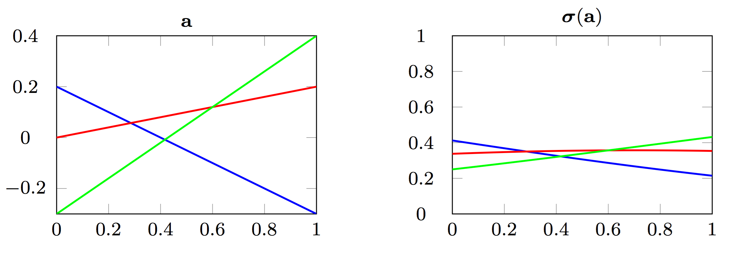] .credit[Figure credit: Y. Avrithis] --- count:false # Softmax - the $\text{softmax}$ function generalizes the sigmoid function and yields a vector of $k$ values in $[0, 1]$ by exponentiating and then normalizing $$\sigma(a) := \text{softmax}(a):= \frac{1}{\sum\_j e^{a\_j}} (e^{a\_1}, \dots, e^{a\_k})$$ - as activation values increase $\text{softmax}$ tends to focus on the maximum .center.width-80[] .credit[Figure credit: Y. Avrithis] --- count:false # Softmax - the $\text{softmax}$ function generalizes the sigmoid function and yields a vector of $k$ values in $[0, 1]$ by exponentiating and then normalizing $$\sigma(a) := \text{softmax}(a):= \frac{1}{\sum\_j e^{a\_j}} (e^{a\_1}, \dots, e^{a\_k})$$ - as activation values increase $\text{softmax}$ tends to focus on the maximum .center.width-80[] .credit[Figure credit: Y. Avrithis] --- count:false # Softmax - the $\text{softmax}$ function generalizes the sigmoid function and yields a vector of $k$ values in $[0, 1]$ by exponentiating and then normalizing $$\sigma(a) := \text{softmax}(a):= \frac{1}{\sum\_j e^{a\_j}} (e^{a\_1}, \dots, e^{a\_k})$$ - as activation values increase $\text{softmax}$ tends to focus on the maximum .center.width-80[] .credit[Figure credit: Y. Avrithis] --- count:false # Softmax - the $\text{softmax}$ function generalizes the sigmoid function and yields a vector of $k$ values in $[0, 1]$ by exponentiating and then normalizing $$\sigma(a) := \text{softmax}(a):= \frac{1}{\sum\_j e^{a\_j}} (e^{a\_1}, \dots, e^{a\_k})$$ - as activation values increase $\text{softmax}$ tends to focus on the maximum .center.width-80[] .credit[Figure credit: Y. Avrithis] --- count:false # Softmax - the $\text{softmax}$ function generalizes the sigmoid function and yields a vector of $k$ values in $[0, 1]$ by exponentiating and then normalizing $$\sigma(a) := \text{softmax}(a):= \frac{1}{\sum\_j e^{a\_j}} (e^{a\_1}, \dots, e^{a\_k})$$ - as activation values increase $\text{softmax}$ tends to focus on the maximum .center.width-80[] .credit[Figure credit: Y. Avrithis] --- count:false # Softmax - the $\text{softmax}$ function generalizes the sigmoid function and yields a vector of $k$ values in $[0, 1]$ by exponentiating and then normalizing $$\sigma(a) := \text{softmax}(a):= \frac{1}{\sum\_j e^{a\_j}} (e^{a\_1}, \dots, e^{a\_k})$$ - as activation values increase $\text{softmax}$ tends to focus on the maximum .center.width-80[] .credit[Figure credit: Y. Avrithis] --- class: middle .center.width-50[] --- count:false # Why stacking layers is a good idea? .grid[ .kol-4-12[ .center.width-100[] .caption[The toy spiral data consists of three classes (blue, red, yellow) that are not linearly separable.] ] .kol-4-12[] .kol-4-12[] ] --- # Why stacking layers is a good idea? .grid[ .kol-4-12[ .center.width-100[] .caption[The toy spiral data consists of three classes (blue, red, yellow) that are not linearly separable.] ] .kol-4-12[ .center.width-100[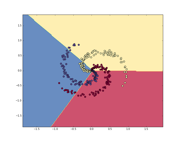] .caption[Linear classifier fails to learn the toy spiral dataset.] ] .kol-4-12[] ] --- # Why stacking layers is a good idea? .grid[ .kol-4-12[ .center.width-100[] .caption[The toy spiral data consists of three classes (blue, red, yellow) that are not linearly separable.] ] .kol-4-12[ .center.width-100[] .caption[Linear classifier fails to learn the toy spiral dataset.] ] .kol-4-12[ .center.width-100[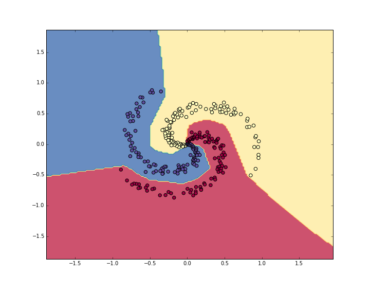] .caption[2 layer neural network manages to solve it] ] ] --- # Backpropagation Consider a 1-dimensional output composition $f \circ g$, such that $$\begin{aligned} y &= f(\mathbf{u}) \\\\ \mathbf{u} &= g(x) = (g\_1(x), ..., g\_m(x)). \end{aligned}$$ The **chain rule** of total derivatives states that $$\frac{\text{d} y}{\text{d} x} = \sum\_{k=1}^m \frac{\partial y}{\partial u\_k} \underbrace{\frac{\text{d} u\_k}{\text{d} x}}\_{\text{recursive case}}$$ - Since a neural network is a composition of differentiable functions, the total derivatives of the loss can be evaluated by applying the chain rule recursively over its computational graph. - The implementation of this procedure is called (reverse) **automatic differentiation** (AD). .credit[Slide credit: G. Louppe] --- As a guiding example, let us consider a simplified 2-layer MLP and the following loss function: $$\begin{aligned} f(\mathbf{x}; \mathbf{W}\_1, \mathbf{W}\_2) &= \sigma\left( \mathbf{W}\_2^T \sigma\left( \mathbf{W}\_1^T \mathbf{x} \right)\right) \\\\ \mathcal{\ell}(y, \hat{y}; \mathbf{W}\_1, \mathbf{W}\_2) &= \text{cross\\_entropy}(y, \hat{y}) + \lambda \left( ||\mathbf{W}_1||\_2 + ||\mathbf{W}\_2||\_2 \right) \end{aligned}$$ for $\mathbf{x} \in \mathbb{R^p}$, $y \in \mathbb{R}$, $\mathbf{W}\_1 \in \mathbb{R}^{p \times q}$ and $\mathbf{W}\_2 \in \mathbb{R}^q$. .credit[Slide credit: G. Louppe] -- .center.width-60[<img src="images/part3/backprop1.png">] --- The total derivative $\frac{\text{d} \ell}{\text{d} \mathbf{W}\_1}$ can be computed **backward**, by walking through all paths from $\ell$ to $\mathbf{W}\_1$ in the computational graph and accumulating the terms: $$\begin{aligned} \frac{\text{d} \ell}{\text{d} \mathbf{W}\_1} &= \frac{\partial \ell}{\partial u\_8}\frac{\text{d} u\_8}{\text{d} \mathbf{W}\_1} + \frac{\partial \ell}{\partial u\_4}\frac{\text{d} u\_4}{\text{d} \mathbf{W}\_1} \\\\ \frac{\text{d} u\_8}{\text{d} \mathbf{W}\_1} &= ... \end{aligned}$$ .center.width-60[<img src="images/part3/backprop2.png">] .credit[Slide credit: G. Louppe] --- # Today ## Convolutional networks ## Siamese and triplet networks --- class: center, middle # Convolutional layers --- # Why would we need them? If they were handled as normal "unstructured" vectors, large-dimension signals such as sound samples or images would require models of intractable size. For instance a linear layer taking a $256 \times 256$ RGB image as input, and producing an image of same size would require: $$ (256 \times 256 \times 3)ˆ2 \simeq 3.87e+10$$ parameters, with the corresponding memory footprint ($\simeq$150Gb !), and excess of capacity. -- .center.width-40[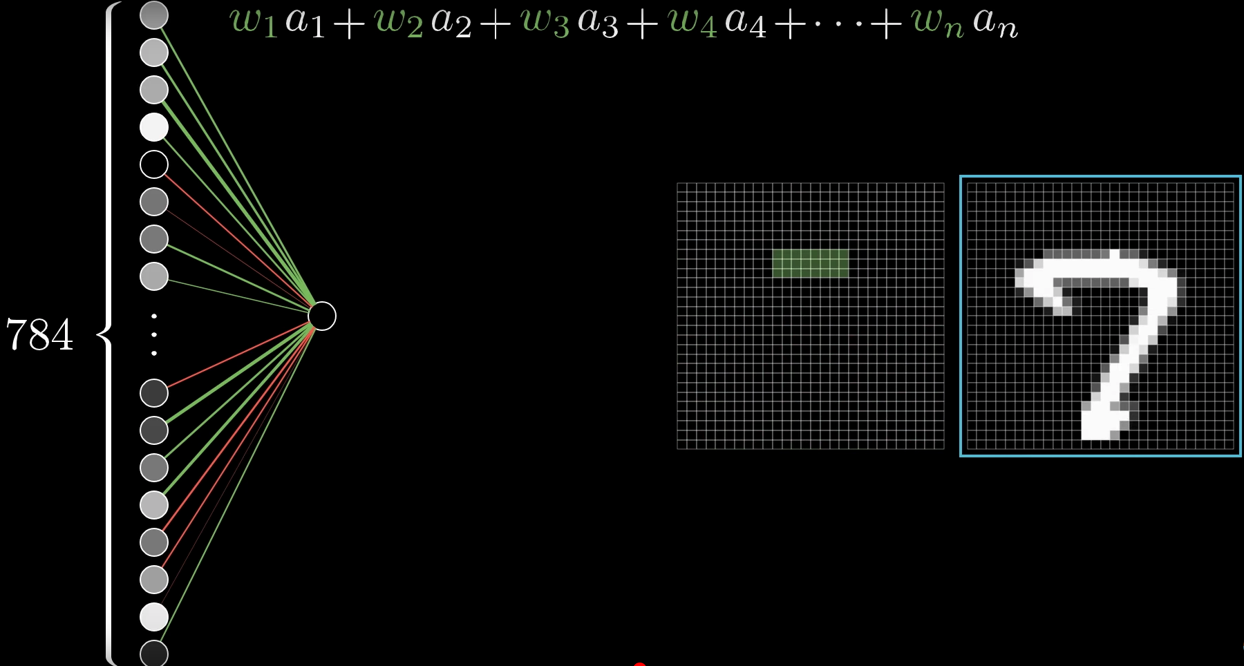] --- # Why would we need them? Moreover, this requirement is inconsistent with the intuition that such large signals have some "invariance in translation". __A representation meaningful at a certain location can / should be used everywhere.__ .credit[Slide credit: F. Fleuret] --- # Why would we need them? Moreover, this requirement is inconsistent with the intuition that such large signals have some "invariance in translation". __A representation meaningful at a certain location can / should be used everywhere.__ A convolutional layer embodies this idea. It applies the same linear transformation locally, everywhere, and preserves the signal structure. .credit[Slide credit: F. Fleuret] --- # Why would we need them? - One neuron gets specialized for detecting a full-image pattern, while being sensible to translations .center.width-70[] --- # Why would we need them? - Each neuron gets specialized for detecting a full-image pattern. - Neurons from later layer work similarly - This is a big waste of parameters without good performance. .center.width-40[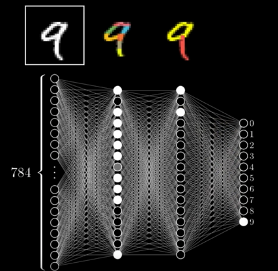] --- # Why would we need them? .center.width-100[] --- # Why would we need them? .center.width-70[] --- class: middle, black-slide .center.width-100[] --- # Fully connected layer .center.width-30[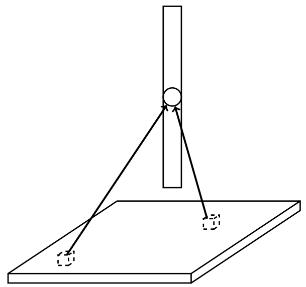] In a **fully connected layer**, each hidden unit $h\_j = \sigma(\mathbf{w}\_j^T \mathbf{x}+b\_j)$ is connected to the entire image. - Looking for activations that depend on pixels that are spatially far away is supposedly a waste of time and resources. - Long range correlations can be dealt with in the higher layers. --- # Locally connected layer .center.width-30[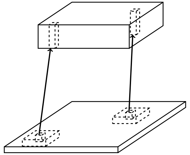] In a **locally connected layer**, each hidden unit $h\_j$ is connected to only a patch of the image. - Weights are specialized locally and functionally. - Reduce the number of parameters. - What if the object in the image shifts a little? --- # Convolutional layer .center.width-30[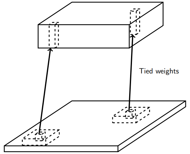] In a **convolutional layer**, each hidden unit $h\_j$ is connected to only a patch of the image, and **share** its weights with the other units $h\_i$. - Weights are specialized functionally, regardless of spatial location. - Reduce the number of parameters. --- # Convolution For one-dimensional tensors, given an input vector $\mathbf{x} \in \mathbb{R}^W$ and a convolutional kernel $\mathbf{u} \in \mathbb{R}^w$, the discrete **convolution** $\mathbf{x} \star \mathbf{u}$ is a vector of size $W - w + 1$ such that $$\begin{aligned} (\mathbf{x} \star \mathbf{u})\_i &= \sum\_{m=0}^{w-1} x\_{i+m} u\_m . \end{aligned} $$ Technically, $\star$ denotes the cross-correlation operator. However, most machine learning libraries call it convolution. --- # Convolution 1d .center.width-60[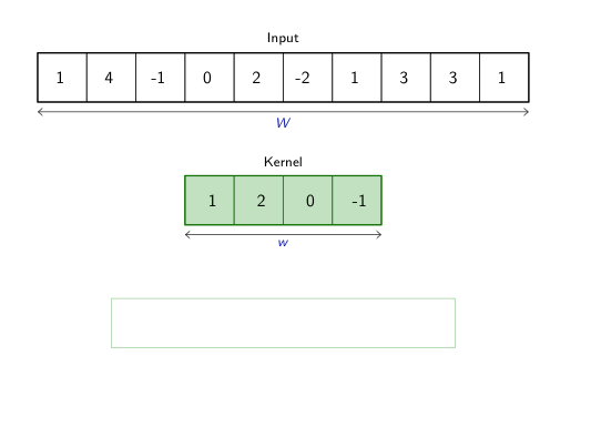] .credit[Slide credit: F. Fleuret] --- count: false # Convolution 1d .center.width-60[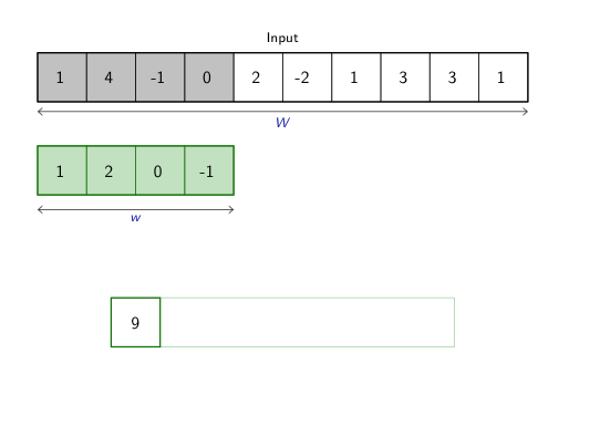] .credit[Slide credit: F. Fleuret] --- count: false # Convolution 1d .center.width-60[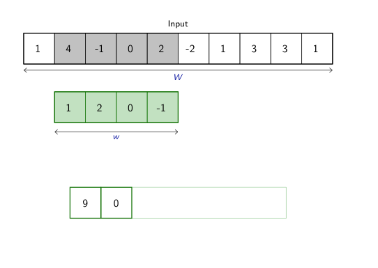] .credit[Slide credit: F. Fleuret] --- count: false # Convolution 1d .center.width-60[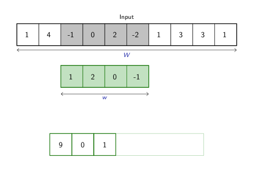] .credit[Slide credit: F. Fleuret] --- count: false # Convolution 1d .center.width-60[] .credit[Slide credit: F. Fleuret] --- count: false # Convolution 1d .center.width-60[] .credit[Slide credit: F. Fleuret] --- count: false # Convolution 1d .center.width-60[] .credit[Slide credit: F. Fleuret] --- count: false # Convolution 1d .center.width-60[] .credit[Slide credit: F. Fleuret] --- count: false # Convolution 1d .center.width-60[] .credit[Slide credit: F. Fleuret] --- # Convolution Convolutions generalize to multi-dimensional tensors: - In its most usual form, a convolution takes as input a 3D tensor $\mathbf{x} \in \mathbb{R}^{C \times H \times W}$, called the input feature map. - A kernel $\mathbf{u} \in \mathbb{R}^{C \times h \times w}$ slides across the input feature map, along its height and width. The size $h \times w$ is called the receptive field. - At each location, the element-wise product between the kernel and the input elements it overlaps is computed and the results are summed up. --- # Convolution - The final output $\mathbf{o}$ is a 2D tensor of size $(H-h+1) \times (W-w+1)$ called the output feature map and such that: $$\begin{aligned} \mathbf{o}\_{j,i} &= \mathbf{b}\_{j,i} + \sum\_{c=0}^{C-1} (\mathbf{x}\_c \star \mathbf{u}\_c)\_{j,i} = \mathbf{b}\_{j,i} + \sum\_{c=0}^{C-1} \sum\_{n=0}^{h-1} \sum\_{m=0}^{w-1} \mathbf{x}\_{c,j+n,i+m} \mathbf{u}\_{c,n,m} \end{aligned}$$ where $\mathbf{u}$ and $\mathbf{b}$ are shared parameters to learn. - $D$ convolutions can be applied in the same way to produce a $D \times (H-h+1) \times (W-w+1)$ feature map, where $D$ is the depth. --- # Convolution 2d .center.width-60[] .credit[Slide credit: F. Fleuret] --- count: false # Convolution 2d .center.width-60[] .credit[Slide credit: F. Fleuret] --- count: false # Convolution 2d .center.width-60[] .credit[Slide credit: F. Fleuret] --- count: false # Convolution 2d .center.width-60[] .credit[Slide credit: F. Fleuret] --- count: false # Convolution 2d .center.width-60[] .credit[Slide credit: F. Fleuret] --- count: false # Convolution 2d .center.width-60[] .credit[Slide credit: F. Fleuret] --- count: false # Convolution 2d .center.width-60[] .credit[Slide credit: F. Fleuret] --- count: false # Convolution 2d .center.width-60[] .credit[Slide credit: F. Fleuret] --- count: false # Convolution 2d .center.width-60[] .credit[Slide credit: F. Fleuret] --- count: false # Convolution 2d .center.width-60[] .credit[Slide credit: F. Fleuret] --- count: false # Convolution 2d .center.width-60[] .credit[Slide credit: F. Fleuret] --- count: false # Convolution 2d .center.width-60[] .credit[Slide credit: F. Fleuret] --- count: false # Convolution 2d .center.width-60[] .credit[Slide credit: F. Fleuret] --- # Image kernels explained visually .center.width-80[] .citation[url: http://setosa.io/ev/image-kernels/] --- # Channels Colored image = tensor of shape `(height, width, channels)` -- Convolutions can be computed across channels: .center[ <img src="images/part3/convmap1_dims.svg" style="width: 300px;" /> ] -- $$ (im \star k)\_{j,i} = \sum\limits\_{c=0}^2 \sum\limits\_{n=0}^4 \sum\limits\_{m=0}^4 im\_{j + n - 2, i + m - 2, c} k\_{n, m, c} $$ --- # Channels - For first layer, RGB channels of input image can be easily visualized - Number of channels is typically increased at deeper levels of the network .center[ <img src="images/part3/conv_rgb.png" style="width: 500px;" /> ] --- # Convolutions as neurons - Since convolutions output one scalar at a time, they can be seen as an individual neuron from a MLP with a receptive field limited to the dimensions of the kernel - The same neuron is "fired" over multiple areas from the input. .center[ <img src="images/part3/conv_intuition_1.png" style="width: 600px;" /> ] --- # Convolutions as neurons - Since convolutions output one scalar at a time, they can be seen as an individual neuron from a MLP with a receptive field limited to the dimensions of the kernel - The same neuron is "fired" over multiple areas from the input. .left-column[ <br> .center[ <img src="images/part3/conv_intuition_1.png" style="width: 350px;" /> ] ] .right-column[ .center[.green[Remember this?]] .center[ <img src="images/part3/neuron_1.png" style="width: 350px;" /> ] ] --- # Convolutions as neurons - Since convolutions output one scalar at a time, they can be seen as an individual neuron from a MLP with a receptive field limited to the dimensions of the kernel - The same neuron is "fired" over multiple areas from the input. .left-column[ <br> .center[ <img src="images/part3/conv_intuition_2.png" style="width: 350px;" /> ] ] .right-column[ .center[.green[Remember this?]] .center[ <img src="images/part3/neuron_1.png" style="width: 350px;" /> ] ] --- class: middle We usually refer to one of the channels generated by a convolution layer as an __activation map__. The sub-area of an input map that influences a component of the output as the __receptive field__ of the latter. In the context of convolutional networks, a standard linear layer is called a __fully connected layer__ since every input influences every output. # Strides - Strides: increment step size for the convolution operator - Reduces the size of the ouput map .center[ <img src="images/part3/no_padding_strides.gif" style="width: 260px;" /> ] .caption[ Example with kernel size $3 \times 3$ and a stride of $2$ (image in blue) ] --- # Padding - Padding: artifically fill borders of image - Useful to keep spatial dimension constant across filters - Useful with strides and large receptive fields - Usually: fill with 0s .center[ <img src="images/part3/same_padding_no_strides.gif" style="width: 260px;" /> ] --- count: false # Padding - Example: input $C \times 3 \times 5$ .center[ <img src="images/part3/padding_1.png" style="width: 400px;" /> ] .credit[Figure credit: F. Fleuret] --- count: false # Padding - Example: input $C \times 3 \times 5$, padding of $(2,1)$ .center[ <img src="images/part3/padding_2.png" style="width: 400px;" /> ] .credit[Figure credit: F. Fleuret] --- count: false # Padding - Example: input $C \times 3 \times 5$, padding of $(2,1)$, a stride of $(2,2)$ .center[ <img src="images/part3/padding_3.png" style="width: 400px;" /> ] .credit[Figure credit: F. Fleuret] --- count: false # Padding - Example: input $C\times3\times5$, padding of $(2,1)$, a stride of $(2,2)$, kernel of size $C\times3\times5$ .center[ <img src="images/part3/padding_4.png" style="width: 400px;" /> ] .credit[Figure credit: F. Fleuret] --- count: false # Padding - Example: input $C\times3\times5$, padding of $(2,1)$, a stride of $(2,2)$, kernel of size $C\times3\times5$ .center[ <img src="images/part3/padding_5.png" style="width: 400px;" /> ] .credit[Figure credit: F. Fleuret] --- count: false # Padding - Example: input $C\times3\times5$, padding of $(2,1)$, a stride of $(2,2)$, kernel of size $C\times3\times5$ .center[ <img src="images/part3/padding_6.png" style="width: 400px;" /> ] .credit[Figure credit: F. Fleuret] --- count: false # Padding - Example: input $C\times3\times5$, padding of $(2,1)$, a stride of $(2,2)$, kernel of size $C\times3\times5$ .center[ <img src="images/part3/padding_7.png" style="width: 400px;" /> ] .credit[Figure credit: F. Fleuret] --- count: false # Padding - Example: input $C\times3\times5$, padding of $(2,1)$, a stride of $(2,2)$, kernel of size $C\times3\times5$ .center[ <img src="images/part3/padding_8.png" style="width: 400px;" /> ] .credit[Figure credit: F. Fleuret] --- count: false # Padding - Example: input $C\times3\times5$, padding of $(2,1)$, a stride of $(2,2)$, kernel of size $C\times3\times5$ .center[ <img src="images/part3/padding_9.png" style="width: 400px;" /> ] .credit[Figure credit: F. Fleuret] --- count: false # Padding - Example: input $C\times3\times5$, padding of $(2,1)$, a stride of $(2,2)$, kernel of size $C\times3\times5$ .center[ <img src="images/part3/padding_10.png" style="width: 400px;" /> ] .credit[Figure credit: F. Fleuret] --- count: false # Padding - Example: input $C\times3\times5$, padding of $(2,1)$, a stride of $(2,2)$, kernel of size $C\times3\times5$ .center[ <img src="images/part3/padding_11.png" style="width: 400px;" /> ] .credit[Figure credit: F. Fleuret] --- count: false # Padding - Example: input $C\times3\times5$, padding of $(2,1)$, a stride of $(2,2)$, kernel of size $C\times3\times5$ .center[ <img src="images/part3/padding_12.png" style="width: 400px;" /> ] .credit[Figure credit: F. Fleuret] --- count: false # Padding - Example: input $C\times3\times5$, padding of $(2,1)$, a stride of $(2,2)$, kernel of size $C\times3\times5$ .center[ <img src="images/part3/padding_13.png" style="width: 400px;" /> ] .credit[Figure credit: F. Fleuret] --- count: false # Padding - Example: input $C\times3\times5$, padding of $(2,1)$, a stride of $(2,2)$, kernel of size $C\times3\times5$ .center[ <img src="images/part3/padding_13.png" style="width: 400px;" /> ] - Pooling operations have a default stride equal to their kernel size, and convolutions have a default stride of 1. - Padding can be useful to generate an output of same size as the input. .credit[Figure credit: F. Fleuret] --- <br> .big[ ```py torch.nn.functional.conv2d(input, weight, bias=None, stride=1, padding=0, dilation=1, groups=1) ``` ] Implements a 2d convolution, where _weight_ contains the kernels, and is $D \times C \times h \times w$, _bias_ is of dimension $D$, _input_ is of dimension $$N \times C \times H \times W $$ and the result is of dimension: $$ N \times D \times (H-h+1) \times (W-w+1) $$ ``` >>> weight = torch.empty(5, 4, 2, 3).normal_() >>> bias = torch.empty(5).normal_() >>> input = torch.empty(117, 4, 10, 3).normal_() >>> output = torch.nn.functional.conv2d(input, weight, bias) >>> output.size() torch.Size([117, 5, 9, 1]) ``` -- Similar functions implements 1d and 3d convolutions. --- <br> .big[```py class torch.nn.Conv2d(in_channels, out_channels, kernel_size, stride=1, padding=0, dilation=1, groups=1, bias=True) ```] Wraps the convolution into a _Module_, with the kernel and biases as _Parameter_ properly randomized at creation. The kernel size is either a pair $(h,w)$ or a single value $k$ interpreted as $(k,k)$. -- ```py >>> f = nn.Conv2d(in_channels = 4, out_channels = 5, kernel_size = (2, 3)) >>> for n, p in f.named_parameters(): print(n, p.size()) ... weight torch.Size([5, 4, 2, 3]) bias torch.Size([5]) >>> x = torch.empty(117, 4, 10, 3).normal_() >>> y = f(x) >>> y.size() torch.Size([117, 5, 9, 1]) ``` --- --- # Convolutions explained visually .center.width-30[] .citation[url: https://ezyang.github.io/convolution-visualizer/index.html] --- # Dealing with shapes Kernel shape $(F, F, C^i, C^o)$ .left-column[ - $F \times F$ kernel size, - $C^i$ input channels - $C^o$ output channels ] .right-column[ .center[ <img src="images/part3/kernel.svg" style="width: 100px;" /> ] ] -- .reset-column[ ] Number of parameters: $(F \times F \times C^i + 1) \times C^o$ -- Activation shapes: - Input $(W^i, H^i, C^i)$ - Output $(W^o, H^o, C^o)$ -- $W^o = (W^i - F + 2P) / S + 1$ .credit[Slide credit: C. Ollion & O. Grisel] --- # Convolutions 1x1 convolution layers: aggregating pixel information from all feature maps <br/> .center[ <img src="images/part3/conv_1x1.png" style="width: 600px;" /> ] --- # Convolutions - A bank of 256 filters (learned from data) - Each filter is 1d (it applies to a grayscale image) - Each filter is 16 x 16 pixels .center[ <img src="images/part3/conv_example_1.png" style="width: 600px;" /> ] --- # Convolutions - A bank of 256 filters (learned from data) - 3D filters for RGB inputs .center[ <img src="images/part3/conv_example_2.png" style="width: 600px;" /> ] --- # Downsampling - Downsampling by a factor $S$ amount to keeping only one every $S$ pixels, discarding others - Filter banks often incorporate or are followed by __2x__ output downsampling - Downsampling is often matched with an increase in the number of feature channels - Overall the volume of the tensors decreases slowly .center[ <img src="images/part3/downsampling.png" style="width: 500px;" /> ] --- # Spatial pooling .center[ <img src="images/part3/spatial_pooling.png" style="width: 500px;" /> ] --- # Pooling - Spatial dimension reduction - Local invariance - No parameters: max or average of 2x2 units .center[ <img src="images/part3/pooling.png" style="width: 560px;" /> ] --- # Pooling - Spatial dimension reduction - Local invariance - No parameters: max or average of 2x2 units .center[ <img src="images/part3/maxpool.svg" style="width: 380px;" /> ] --- # Max-Pooling 1d .center[ <img src="images/part3/maxpool1d_1.png" style="width: 600px;" /><br/> ] .credit[Slide credit: F. Fleuret] --- count: false # Max-Pooling 1d .center[ <img src="images/part3/maxpool1d_2.png" style="width: 600px;" /><br/> ] .credit[Slide credit: F. Fleuret] --- count: false # Max-Pooling 1d .center[ <img src="images/part3/maxpool1d_3.png" style="width: 600px;" /><br/> ] .credit[Slide credit: F. Fleuret] --- count: false # Max-Pooling 1d .center[ <img src="images/part3/maxpool1d_4.png" style="width: 600px;" /><br/> ] .credit[Slide credit: F. Fleuret] --- count: false # Max-Pooling 1d .center[ <img src="images/part3/maxpool1d_5.png" style="width: 600px;" /><br/> ] .credit[Slide credit: F. Fleuret] --- count: false # Max-Pooling 1d .center[ <img src="images/part3/maxpool1d_6.png" style="width: 600px;" /><br/> ] .credit[Slide credit: F. Fleuret] --- count: false # Max-Pooling 1d .center[ <img src="images/part3/maxpool1d_7.png" style="width: 600px;" /><br/> ] .credit[Slide credit: F. Fleuret] --- # Max-Pooling 2d .center[ <img src="images/part3/maxpool2d_1.png" style="width: 600px;" /><br/> ] .credit[Slide credit: F. Fleuret] --- count: false # Max-Pooling 2d .center[ <img src="images/part3/maxpool2d_2.png" style="width: 600px;" /><br/> ] .credit[Slide credit: F. Fleuret] --- count: false # Max-Pooling 2d .center[ <img src="images/part3/maxpool2d_3.png" style="width: 600px;" /><br/> ] .credit[Slide credit: F. Fleuret] --- count: false # Max-Pooling 2d .center[ <img src="images/part3/maxpool2d_4.png" style="width: 600px;" /><br/> ] .credit[Slide credit: F. Fleuret] --- count: false # Max-Pooling 2d .center[ <img src="images/part3/maxpool2d_5.png" style="width: 600px;" /><br/> ] .credit[Slide credit: F. Fleuret] --- count: false # Max-Pooling 2d .center[ <img src="images/part3/maxpool2d_6.png" style="width: 600px;" /><br/> ] .credit[Slide credit: F. Fleuret] --- count: false # Max-Pooling 2d .center[ <img src="images/part3/maxpool2d_7.png" style="width: 600px;" /><br/> ] .credit[Slide credit: F. Fleuret] --- count: false # Max-Pooling 2d .center[ <img src="images/part3/maxpool2d_8.png" style="width: 600px;" /><br/> ] .credit[Slide credit: F. Fleuret] --- count: false # Max-Pooling 2d .center[ <img src="images/part3/maxpool2d_9.png" style="width: 600px;" /><br/> ] .credit[Slide credit: F. Fleuret] --- count: false # Max-Pooling 2d .center[ <img src="images/part3/maxpool2d_10.png" style="width: 600px;" /><br/> ] .credit[Slide credit: F. Fleuret] --- count: false # Max-Pooling 2d .center[ <img src="images/part3/maxpool2d_11.png" style="width: 600px;" /><br/> ] .credit[Slide credit: F. Fleuret] --- count: false # Max-Pooling 2d .center[ <img src="images/part3/maxpool2d_12.png" style="width: 600px;" /><br/> ] .credit[Slide credit: F. Fleuret] --- count: false # Max-Pooling 2d .center[ <img src="images/part3/maxpool2d_13.png" style="width: 600px;" /><br/> ] .credit[Slide credit: F. Fleuret] --- count: false # Max-Pooling 2d .center[ <img src="images/part3/maxpool2d_14.png" style="width: 600px;" /><br/> ] .credit[Slide credit: F. Fleuret] --- count: false # Max-Pooling 2d .center[ <img src="images/part3/maxpool2d_15.png" style="width: 600px;" /><br/> ] .credit[Slide credit: F. Fleuret] --- # Translation invariance from pooling .center[ <img src="images/part3/invariance_1.png" style="width: 500px;" /><br/> ] .credit[Slide credit: F. Fleuret] --- count: false # Translation invariance from pooling .center[ <img src="images/part3/invariance_2.png" style="width: 500px;" /><br/> ] .credit[Slide credit: F. Fleuret] --- count: false # Translation invariance from pooling .center[ <img src="images/part3/invariance_3.png" style="width: 500px;" /><br/> ] .credit[Slide credit: F. Fleuret] --- count: false # Translation invariance from pooling .center[ <img src="images/part3/invariance_4.png" style="width: 500px;" /><br/> ] .credit[Slide credit: F. Fleuret] --- count: false # Translation invariance from pooling .center[ <img src="images/part3/invariance_5.png" style="width: 500px;" /><br/> ] .credit[Slide credit: F. Fleuret] --- <br> .big[ ```py torch.nn.functional.max_pool2d(input, kernel_size, stride=None, padding=0, dilation=1, ceil_mode=False, return_indices=False) ``` ] takes as input a $N \times C \times H \times W$ tensor, and a kernel size $(h,w)$ or $k$ interpreted as $(k,k)$. applies the max-pooling on each channel of each sample separately, and produce if the padding is $0$ a $N \times C \times \lfloor H/h \rfloor \times \lfloor W/w \rfloor$ output. -- ```py >>> x = torch.empty(2, 2, 6).random_(3) >>> x tensor([[[ 1., 2., 2., 1., 2., 1.], [ 2., 0., 0., 0., 1., 0.]], [[ 2., 0., 2., 1., 1., 1.], [ 0., 0., 0., 1., 2., 1.]]]) >>> F.max_pool2d(x, (1, 2)) tensor([[[ 2., 2., 2.], [ 2., 0., 1.]], [[ 2., 2., 1.], [ 0., 1., 2.]]]) ``` Similar function implements 1d and 3d max-pooling, and average pooling --- class: middle As for convolution, pooling operations can be modulated through their stride and padding. While for convolution the default stride is 1, for pooling it is equal to the kernel size, but this not obligatory. Default padding is zero. --- <br> .big[ ```py class torch.nn.MaxPool2d(kernel_size, stride=None, padding=0, dilation=1, return_indices=False, ceil_mode=False) ``` ] Wraps the max-pooling operation into a _Module_. As for convolutions, the kernel size is either a pair $(h,w)$ or a single value $k$ interpreted as $(k,k)$. --- # Layer patterns A **convolutional network** can often be defined as a composition of convolutional layers ($\texttt{CONV}$), pooling layers ($\texttt{POOL}$), linear rectifiers ($\texttt{RELU}$) and fully connected layers ($\texttt{FC}$). <br> .center.width-70[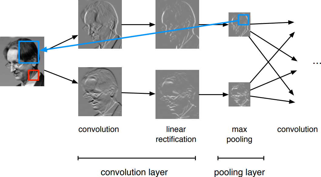] --- class: middle The most common convolutional network architecture follows the pattern: $$\texttt{INPUT} \to [[\texttt{CONV} \to \texttt{RELU}]\texttt{\*}N \to \texttt{POOL?}]\texttt{\*}M \to [\texttt{FC} \to \texttt{RELU}]\texttt{\*}K \to \texttt{FC}$$ where: - $\texttt{\*}$ indicates repetition; - $\texttt{POOL?}$ indicates an optional pooling layer; - $N \geq 0$ (and usually $N \leq 3$), $M \geq 0$, $K \geq 0$ (and usually $K < 3$); - the last fully connected layer holds the output (e.g., the class scores). --- class: middle Some common architectures for convolutional networks following this pattern include: - $\texttt{INPUT} \to \texttt{FC}$, which implements a linear classifier ($N=M=K=0$). - $\texttt{INPUT} \to [\texttt{FC} \to \texttt{RELU}]{\*K} \to \texttt{FC}$, which implements a $K$-layer MLP. - $\texttt{INPUT} \to \texttt{CONV} \to \texttt{RELU} \to \texttt{FC}$. - $\texttt{INPUT} \to [\texttt{CONV} \to \texttt{RELU} \to \texttt{POOL}]\texttt{\*2} \to \texttt{FC} \to \texttt{RELU} \to \texttt{FC}$. - $\texttt{INPUT} \to [[\texttt{CONV} \to \texttt{RELU}]\texttt{\*2} \to \texttt{POOL}]\texttt{\*3} \to [\texttt{FC} \to \texttt{RELU}]\texttt{\*2} \to \texttt{FC}$. Note that for the last architecture, two $\texttt{CONV}$ layers are stacked before every $\texttt{POOL}$ layer. This is generally a good idea for larger and deeper networks, because multiple stacked $\texttt{CONV}$ layers can develop more complex features of the input volume before the destructive pooling operation. --- # ConvNet - Neural network with specialized connectivity structure - Stack multiple stage of feature extractors - Higher stages compute more global, more invariant features - Classification layer at the end <br> .center.width-90[] .citation[LeCun, LeNet-5, 1998] --- # ConvNet .center[.Q[Remember this?]] <br> <br> .width-100[<img src="images/part3/mlp.png" >] .credit[Figure credit: G. Louppe] --- # ConvNet Just like multi-layer perceptorns, convolutional layers can be also composed *in series*, such that: $$\begin{aligned} \mathbf{h}\_0 &= \mathbf{x} \\\\ \mathbf{h}\_1 &= \sigma(\mathbf{W}\_1^T \mathbf{h}\_0 + \mathbf{b}\_1) \\\\ ... \\\\ \mathbf{h}\_L &= \sigma(\mathbf{W}\_L^T \mathbf{h}\_{L-1} + \mathbf{b}\_L) \\\\ f(\mathbf{x}; \theta) &= \mathbf{h}\_L \end{aligned}$$ where $\theta$ denotes the model parameters $\\{ \mathbf{W}\_k, \mathbf{b}\_k, ... | k=1, ..., L\\}$. - Hidden states $\mathbf{h}\_k$ have $2D$ layout and are called _feature maps_ (for MLPs they are $1D$) - Each filter has its own trainable parameters $\mathbf{W}\_k$. - Weights from all filters and layers are trained jointly with backpropagation and gradient descent --- # ConvNet A convolutional layer is composed of convolution, activation and downsampling layers. .center[ <img src="images/part3/conv_layers.png" style="width: 700px;" /><br/> ] --- class: center, middle .width-100[] --- class: center, middle .width-100[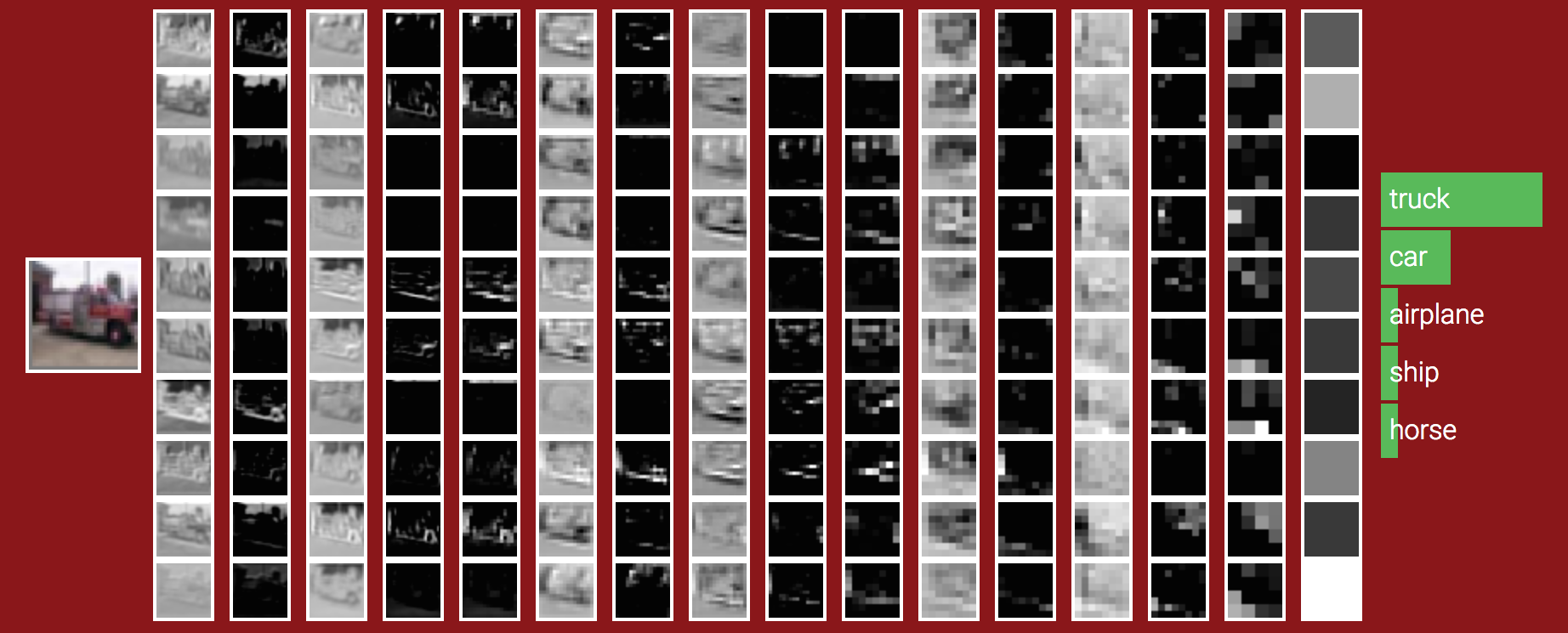] --- # Receptive field - The receptive field is defined as the region in the input space that a particular CNN's feature is looking at (_i.e._ be affected by). - A receptive field of a feature can be fully described by its center location and its size - Example: $k = 3\times3; p = 1\times1; s = 2\times2; input = 3\times3$ .center[ <img src="images/part3/receptive_field_1.png" style="width: 500px;" /> ] .left-column[ .tiny[Common way to visualize a CNN feature map.] ] .right-column[ .tiny[Fixed-sized CNN feature map visualization, where the size of each feature map is fixed, and the feature is located at the center of its receptive field.] ] --- # Receptive field - The receptive field is defined as the region in the input space that a particular CNN's feature is looking at (_i.e._ be affected by). - A receptive field of a feature can be fully described by its center location and its size - Example: $k = 3\times3; p = 1\times1; s = 2\times2; input = 7\times7$ .center[ <img src="images/part3/receptive_field_2.png" style="width: 600px;" /> ] --- # Receptive field - The receptive field is defined as the region in the input space that a particular CNN's feature is looking at (_i.e._ be affected by). - A receptive field of a feature can be fully described by its center location and its size .center[ <img src="images/part3/receptive_field_3.png" style="width: 600px;" /> ] .center[.tiny[Receptive fields for convolutional and pooling layers of VGG-16]] --- class: center, middle # Siamese Networks --- # Siamese networks .center[ <img src="images/part3/lfw.png" style="width: 500px;" /> ] - **Recognition:** given a face, classify among K possible persons - **Verification:** verify that two faces belongs to the same person A verification system can be implemented as a similarity measure. If it's really good, useful for recognition. --- # Siamese architecture .center.width-60[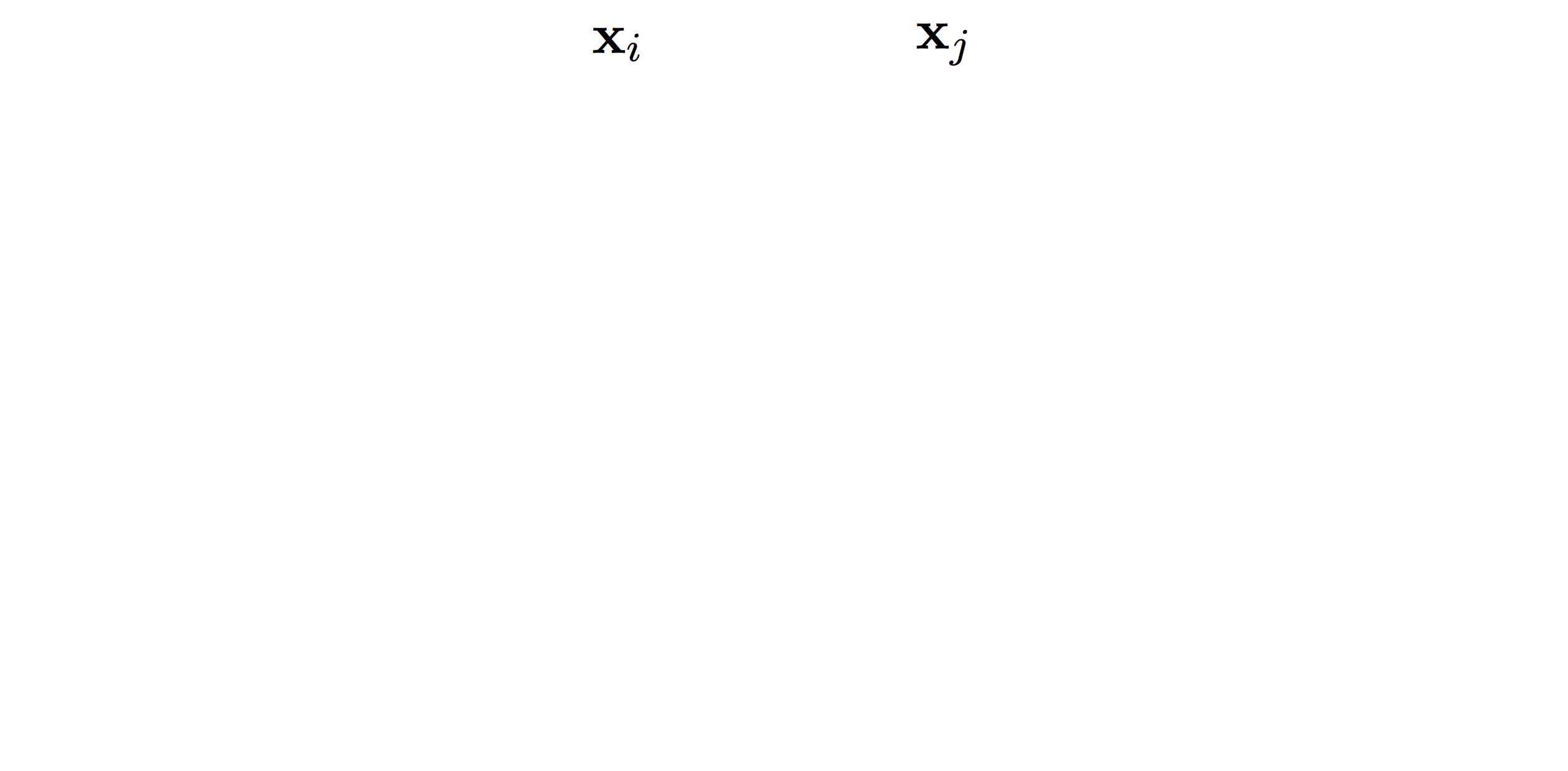] - an input sample is a _pair_ $( \mathbf{x}\_i, \mathbf{x}\_j)$ .citation[ S. Chopra et al.,Learning a similarity metric discriminatively, with application to face verification, CVPR 2005] --- # Siamese architecture .center.width-60[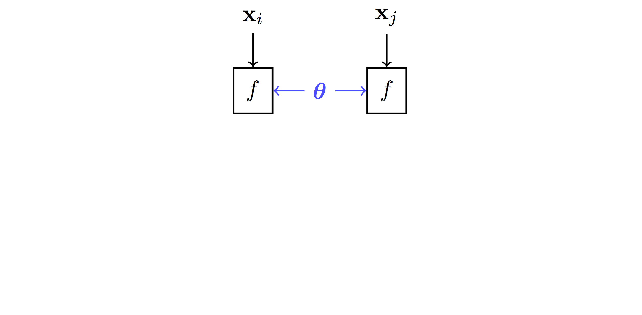] - an input sample is a _pair_ $( \mathbf{x}\_i, \mathbf{x}\_j)$ - both $\mathbf{x}\_i$, $\mathbf{x}\_j$ go through the _same_ function $f$ with _shared_ parameters $\theta$ .citation[ S. Chopra et al.,Learning a similarity metric discriminatively, with application to face verification, CVPR 2005] --- # Siamese architecture .center.width-60[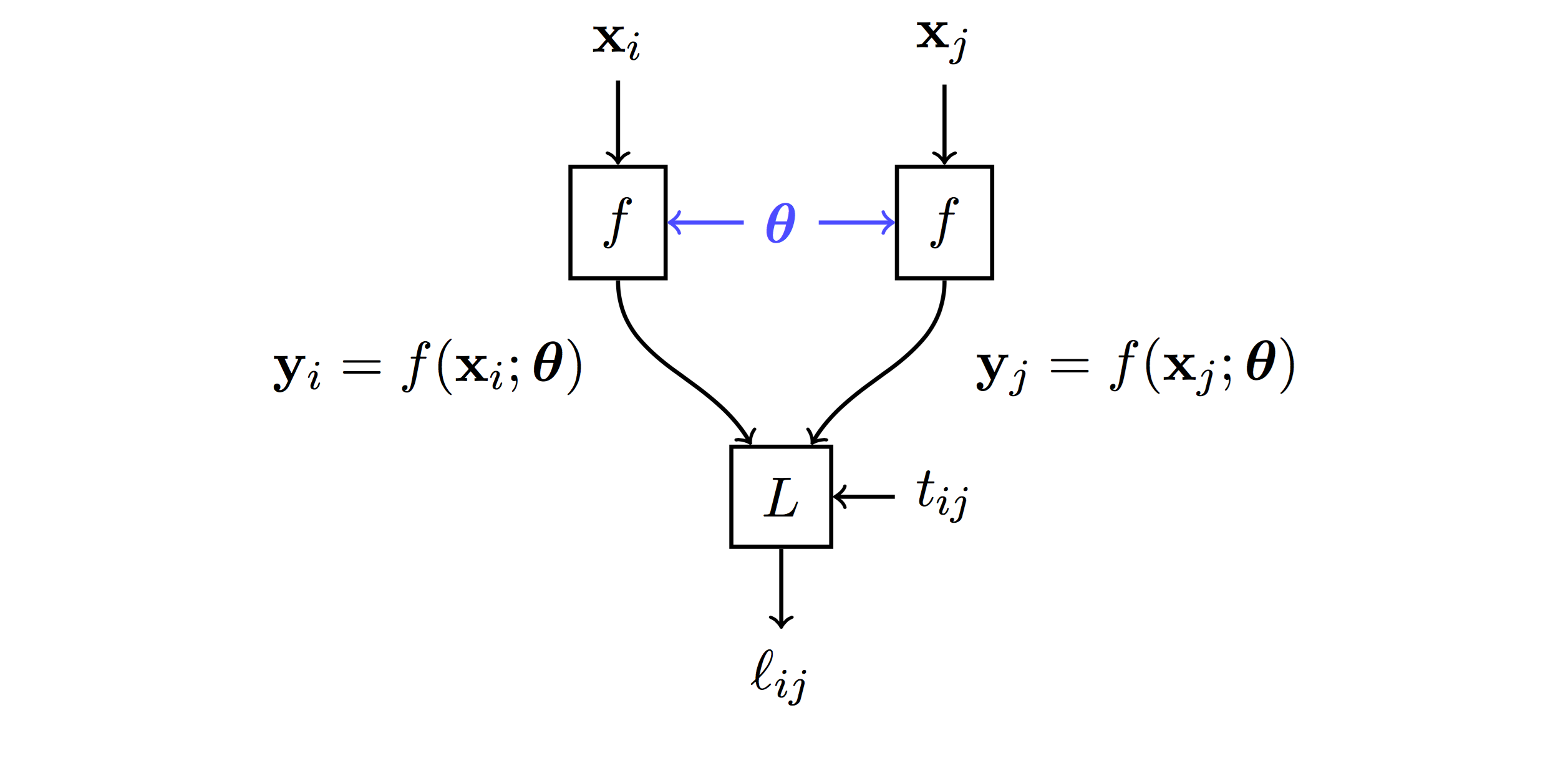] - an input sample is a _pair_ $( \mathbf{x}\_i, \mathbf{x}\_j)$ - both $\mathbf{x}\_i$, $\mathbf{x}\_j$ go through the _same_ function $f$ with _shared_ parameters $\theta$ - loss $\ell\_{ij}$ is measured on output pair $( \mathbf{y}\_i, \mathbf{y}\_j)$ and target $t\_{ij}$ .citation[ S. Chopra et al.,Learning a similarity metric discriminatively, with application to face verification, CVPR 2005] --- # Contrastive loss .center.width-60[] - input samples $\mathbf{x}\_i$, output vectors $\mathbf{y}\_i= f(\mathbf{x}\_i; \theta)$, target variables $t\_{ij}=\mathbb{1}[\text{sim}(\mathbf{x}\_i, \mathbf{x}\_j)]$ - _contrastive loss_ is a function of distance $\Vert \mathbf{y}\_i - \mathbf{y}\_j \Vert$ only $$\ell\_{ij} = L((\mathbf{y}\_i,\mathbf{y}\_j), t\_{ij} ) = \ell (\Vert \mathbf{y}\_i - \mathbf{y}\_j \Vert, t\_{ij})$$ .citation[ R. Hadsell et al., Dimensionality reduction by learning an invariant mapping, CVPR 2006] --- # Contrastive loss .center.width-60[] - input samples $\mathbf{x}\_i$, output vectors $\mathbf{y}\_i= f(\mathbf{x}\_i; \theta)$, target variables $t\_{ij}=\mathbb{1}[\text{sim}(\mathbf{x}\_i, \mathbf{x}\_j)]$ - _contrastive loss_ is a function of distance $\Vert \mathbf{y}\_i - \mathbf{y}\_j \Vert$ only $$\ell\_{ij} = L((\mathbf{y}\_i,\mathbf{y}\_j), t\_{ij} ) = \ell (\Vert \mathbf{y}\_i - \mathbf{y}\_j \Vert, t\_{ij})$$ - _similar_ samples are _attracted_ $$\ell(x,t)=\textcolor{red}{t\ell^{+}} + (1-t)\ell^{-}(x) = \textcolor{red}{t x^2} + (1-t)[m-x]^2\_+$$ .citation[ R. Hadsell et al., Dimensionality reduction by learning an invariant mapping, CVPR 2006] --- # Contrastive loss .center.width-60[] - input samples $\mathbf{x}\_i$, output vectors $\mathbf{y}\_i= f(\mathbf{x}\_i; \theta)$, target variables $t\_{ij}=\mathbb{1}[\text{sim}(\mathbf{x}\_i, \mathbf{x}\_j)]$ - _contrastive loss_ is a function of distance $\Vert \mathbf{y}\_i - \mathbf{y}\_j \Vert$ only $$\ell\_{ij} = L((\mathbf{y}\_i,\mathbf{y}\_j), t\_{ij} ) = \ell (\Vert \mathbf{y}\_i - \mathbf{y}\_j \Vert, t\_{ij})$$ - _dissimilar_ samples are _repelled_ if closer than margin $m$ $$\ell(x,t)=t\ell^{+} + (1-t)\textcolor{red}{\ell^{-}(x)} = t x^2 + (1-t)\textcolor{red}{[m-x]^2\_+}$$ .citation[ R. Hadsell et al., Dimensionality reduction by learning an invariant mapping, CVPR 2006] --- # Triplet architecture .grid[ .kol-6-12[ .center.width-100[] ] .kol-6-12[ - an input sample is a _triple_ $(\mathbf{x}\_i, \mathbf{x}\_i^+, \mathbf{x}\_i^-)$ ] ] .citation[ Wang et al., Learning fine-grained image similarity with deep ranking, CVPR 2014] --- # Triplet architecture .grid[ .kol-6-12[ .center.width-100[] ] .kol-6-12[ - an input sample is a _triple_ $(\mathbf{x}\_i, \mathbf{x}\_i^+, \mathbf{x}\_i^-)$ - $\mathbf{x}\_i, \mathbf{x}\_i^+, \mathbf{x}\_i^-$ go through the _same_ function $f$ with _shared_ parameters $\theta$ ] ] .citation[ Wang et al., Learning fine-grained image similarity with deep ranking, CVPR 2014] --- # Triplet architecture .grid[ .kol-6-12[ .center.width-100[] ] .kol-6-12[ - an input sample is a _triple_ $(\mathbf{x}\_i, \mathbf{x}\_i^+, \mathbf{x}\_i^-)$ - $\mathbf{x}\_i, \mathbf{x}\_i^+, \mathbf{x}\_i^-$ go through the _same_ function $f$ with _shared_ parameters $\theta$ - loss $\ell\_i$ is measured on output triple $(\mathbf{y}\_i, \mathbf{y}\_i^+, \mathbf{y}\_i^-)$ ] ] .citation[ Wang et al., Learning fine-grained image similarity with deep ranking, CVPR 2014] --- # Triplet loss - input _anchor_ $\mathbf{x}\_i$, output vector $\mathbf{y}\_i = f(\mathbf{x}\_i; \theta)$ - positive $\mathbf{y}\_i^+ = f(\mathbf{x}\_i^+; \theta)$, negative $\mathbf{y}\_i^- = f(\mathbf{x}\_i^-; \theta)$ - _triplet loss_ is a function of distances $\Vert \mathbf{y}\_i - \mathbf{y}\_i^+ \Vert$, $\Vert \mathbf{y}\_i - \mathbf{y}\_i^- \Vert$ only $$\ell\_i = L(\mathbf{y}\_i, \mathbf{y}\_i^+, \mathbf{y}\_i^-) =\ell(\Vert \mathbf{y}\_i - \mathbf{y}\_i^+ \Vert, \Vert \mathbf{y}\_i - \mathbf{y}\_i^- \Vert)$$ $$\ell(x^+, x^-) = [m + (x^+)^2 - (x^-)^2]\_+$$ so distance $\Vert \mathbf{y}\_i - \mathbf{y}\_i^+ \Vert$ should be less than $\Vert \mathbf{y}\_i - \mathbf{y}\_i^- \Vert$ by _margin_ $m$ .citation[ Wang et al., Learning fine-grained image similarity with deep ranking, CVPR 2014] --- # Triplet loss - input _anchor_ $\mathbf{x}\_i$, output vector $\mathbf{y}\_i = f(\mathbf{x}\_i; \theta)$ - positive $\mathbf{y}\_i^+ = f(\mathbf{x}\_i^+; \theta)$, negative $\mathbf{y}\_i^- = f(\mathbf{x}\_i^-; \theta)$ - _triplet loss_ is a function of distances $\Vert \mathbf{y}\_i - \mathbf{y}\_i^+ \Vert$, $\Vert \mathbf{y}\_i - \mathbf{y}\_i^- \Vert$ only $$\ell\_i = L(\mathbf{y}\_i, \mathbf{y}\_i^+, \mathbf{y}\_i^-) =\ell(\Vert \mathbf{y}\_i - \mathbf{y}\_i^+ \Vert, \Vert \mathbf{y}\_i - \mathbf{y}\_i^- \Vert)$$ $$\ell(x^+, x^-) = [m + (x^+)^2 - (x^-)^2]\_+$$ so distance $\Vert \mathbf{y}\_i - \mathbf{y}\_i^+ \Vert$ should be less than $\Vert \mathbf{y}\_i - \mathbf{y}\_i^- \Vert$ by _margin_ $m$ - by taking _two pairs_ $(\mathbf{x}\_i, \mathbf{x}\_i^+)$ and $(\mathbf{x}\_i, \mathbf{x}\_i^-)$ at a time with targets $1$, $0$ respectively, the _contrastive loss_ can be writen similarly $$\ell(x^+, x^-) = (x^+)^2 + [m-x^-]^2\_+$$ so distance $\Vert \mathbf{y}\_i - \mathbf{y}\_i^+ \Vert$ should be small and $\Vert \mathbf{y}\_i - \mathbf{y}\_i^- \Vert$ larger than $m$ .citation[ Wang et al., Learning fine-grained image similarity with deep ranking, CVPR 2014] --- # Siamese networks .grid[ .kol-6-12[ ``` class SiameseNet(nn.Module): def __init__(self, embedding_net): super(SiameseNet, self).__init__() self.embedding_net = embedding_net def forward(self, x1, x2): output1 = self.embedding_net(x1) output2 = self.embedding_net(x2) return output1, output2 def get_embedding(self, x): return self.embedding_net(x) ``` ] .kol-6-12[ ``` class TripletNet(nn.Module): def __init__(self, embedding_net): super(TripletNet, self).__init__() self.embedding_net = embedding_net def forward(self, x1, x2, x3): output1 = self.embedding_net(x1) output2 = self.embedding_net(x2) output3 = self.embedding_net(x3) return output1, output2, output3 def get_embedding(self, x): return self.embedding_net(x) ``` ] ] --- count:false # Siamese networks .grid[ .kol-6-12[ ``` class SiameseNet(nn.Module): def __init__(self, embedding_net): super(SiameseNet, self).__init__() self.embedding_net = embedding_net def forward(self, x1, x2): * output1 = self.embedding_net(x1) * output2 = self.embedding_net(x2) return output1, output2 def get_embedding(self, x): return self.embedding_net(x) ``` ] .kol-6-12[ ``` class TripletNet(nn.Module): def __init__(self, embedding_net): super(TripletNet, self).__init__() self.embedding_net = embedding_net def forward(self, x1, x2, x3): * output1 = self.embedding_net(x1) * output2 = self.embedding_net(x2) * output3 = self.embedding_net(x3) return output1, output2, output3 def get_embedding(self, x): return self.embedding_net(x) ``` ] ] --- # Hard negative sampling After a few epochs, If $(x\_i, x\_i^{+}, x\_i^{-})$ are chosen randomly, it will be easy to satisfy the inequality in the loss. -- Gradient in one batch quickly become almost $0$ except for **hard cases**. Random sampling is inefficient to find these hard cases -- - **Hard triplet sampling:** sample $x\_i^{-}$ such that: $||f(x\_i) - f(x\_i^{+})||_2 > ||f(x\_i) - f(x\_i^{-})||_2 + \alpha$ - **Semi Hard triplet sampling:** sample $x\_i^{-}$ such that: $||f(x\_i) - f(x\_i^{+})||_2 > ||f(x\_i) - f(x\_i^{-})||_2$ --- # Face recognition .center.width-30[] - A threshold is computed on test set ($1.2$) - Best model achieves 99.6% verification accuracy on LFW - Face alignment is critical! .citation[F. Schroff et al., Facenet: A unified embedding for face recognition and clustering, CVPR 2015 ] --- # Deep image retrieval .center.width-70[] .citation[A. Gordo et al., Deep Image Retrieval: Learning Global Representations for Image Search, ECCV 2016 ] - query $\mathbf{x}\_i$, relevant $\mathbf{x}\_i^+$ (same building), irrelevant $\mathbf{x}\_i^-$ (other building) --- # Deep image retrieval .center.width-70[] .citation[A. Gordo et al., Deep Image Retrieval: Learning Global Representations for Image Search, ECCV 2016 ] - query $\mathbf{x}\_i$, relevant $\mathbf{x}\_i^+$ (same building), irrelevant $\mathbf{x}\_i^-$ (other building) --- # Deep image retrieval .center.width-70[] .citation[A. Gordo et al., Deep Image Retrieval: Learning Global Representations for Image Search, ECCV 2016 ] - query $\mathbf{x}\_i$, relevant $\mathbf{x}\_i^+$ (same building), irrelevant $\mathbf{x}\_i^-$ (other building) - triplet loss is evaluated on output $(\mathbf{y}\_i, \mathbf{y}\_i^+, \mathbf{y}\_i^-)$ --- # Patch matching .center.width-50[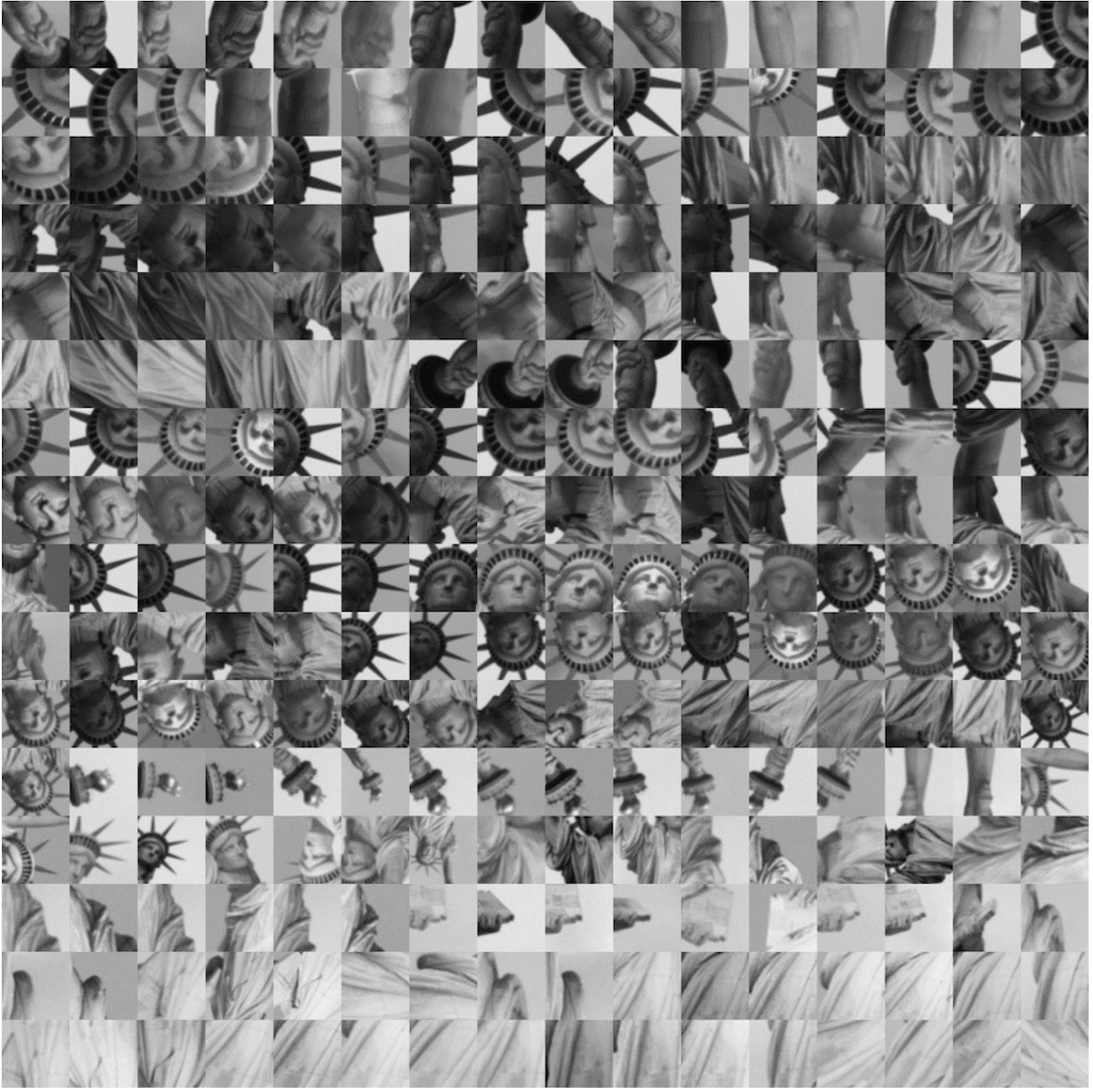] --- # Patch matching .center.width-70[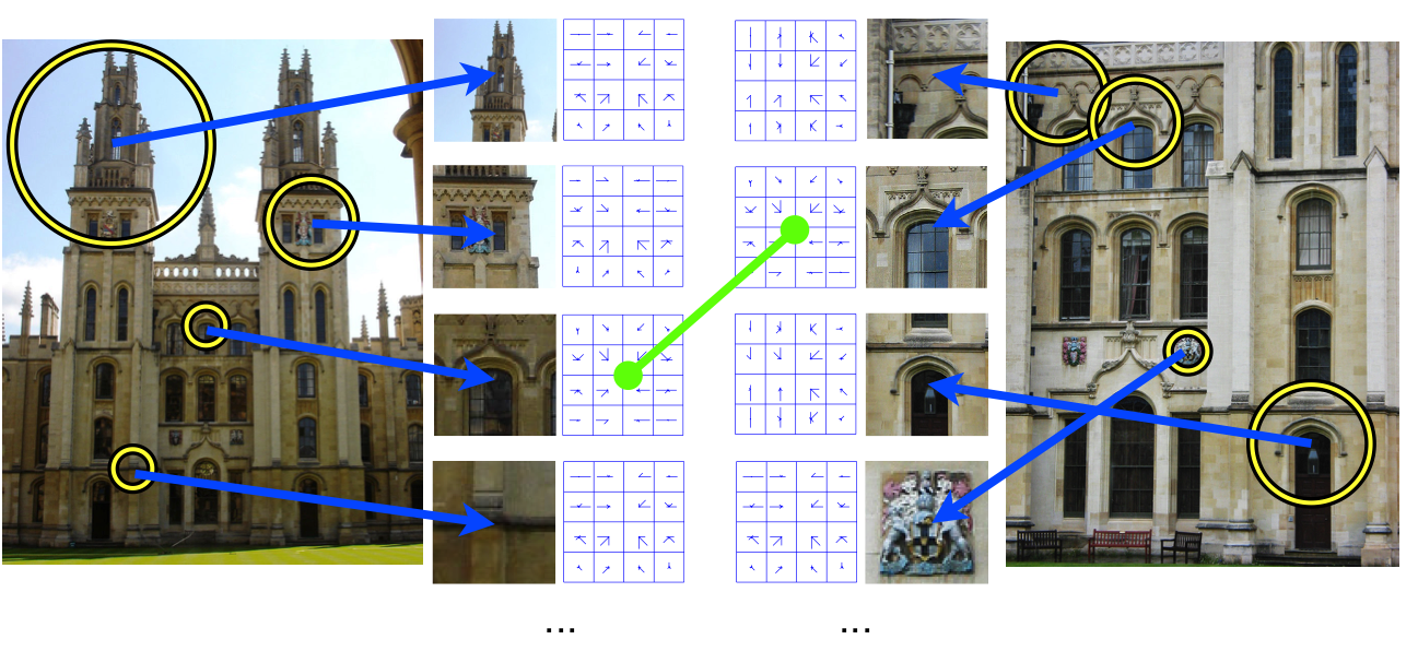] .credit[Figure credit: A. Vedaldi] --- # Patch matching .center.width-60[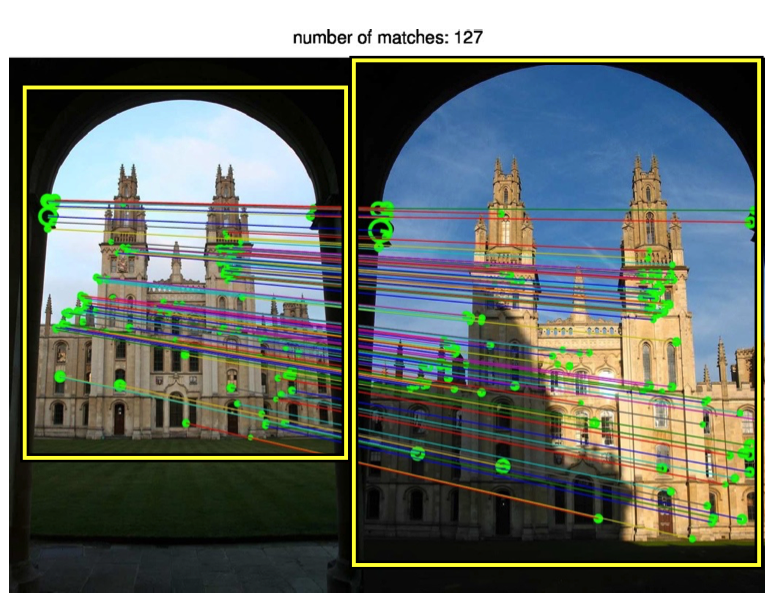] .credit[Figure credit: A. Vedaldi] --- # Image reconstruction .center.width-70[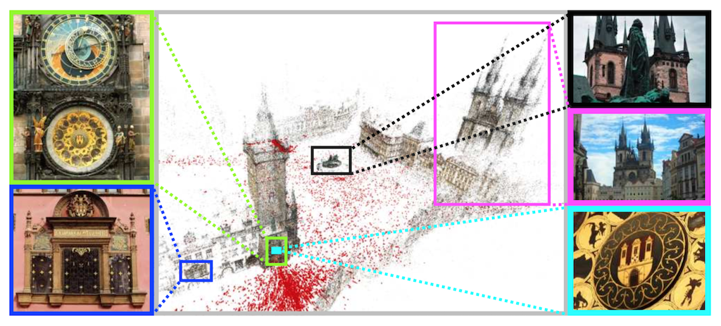] .caption[Structure from motion] .citation[F. Radenovic et al., CNN Image Retrieval Learns From BoW: Unsupervised Fine-Tuning with Hard Examples, ECCV 2016 <br/> Schonberger et al., From Single Image Query to Detailed 3D Reconstruction, CVPR 2015.] --- # Person re-identification .grid[ .kol-6-12[ .center.width-70[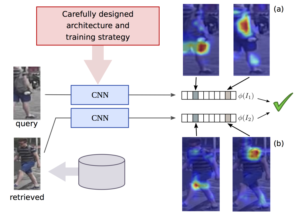] ] .kol-6-12[ ] ] .citation[J. Almazan et al., Re-ID Done Right: towards Good Practices for Person re-Identification, arXiv 2018] --- count: false # Person re-identification .grid[ .kol-6-12[ .center.width-70[] ] .kol-6-12[ .center.width-70[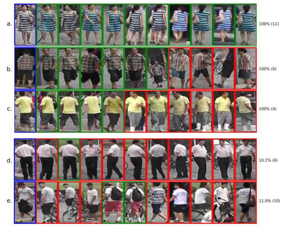] ] ] .citation[J. Almazan et al., Re-ID Done Right: towards Good Practices for Person re-Identification, arXiv 2018] --- class: middle, center ## Few classes, few labels --- # Prototypical networks Learns to extract class prototype vectors: - class prototype vector = mean feature vector of training examples - classify test example to the class with the closest prototype ($L\_2$ distance) - prototype vectors are similar to classification weights of networks .grid[ .kol-6-12[ Prototype vector of $k$-th class: $$c\_k=\frac{1}{|S\_k|} \sum\_{(x\_i, y\_i) \in S\_k} f\_{\theta}(x\_i)$$ Classification for example $x$: $$p\_{\theta}(y=k|x) = \frac{\exp(-d(f\_{\theta}(x), c\_k))}{\sum\_{k'}\exp(-d(f\_{\theta}(x), c\_{k'}))}$$ ] .kol-6-12[ .center.width-70[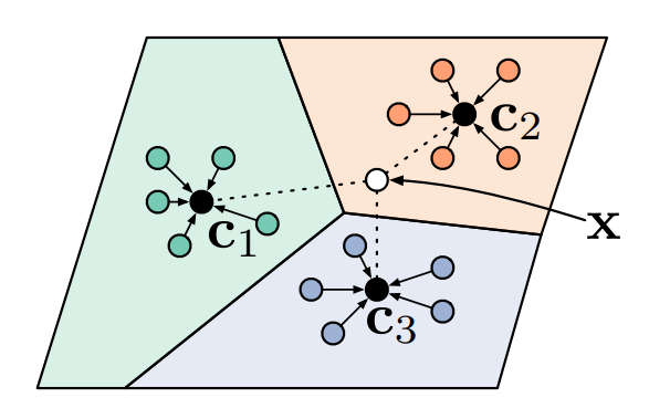] ] ] .citation[J Snell et al., Prototypical Networks for Few-shot Learning, NeurIPS 2017] --- class: middle, center ## Mix of (Few classes, few labels) + (random classes, many label)s --- # Imprinting .left-column[ .center.width-100[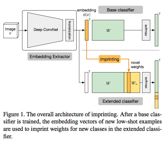] ] .right-column[ ] .citation[H. Qi et al., Low-Shot Learning with Imprinted Weights, CVPR 2018] --- count: false # Imprinting .left-column[ .center.width-100[] ] .right-column[ .center.width-100[] .caption[ _left_: before imprinting; _right_: after imprinting] ] .citation[H. Qi et al., Low-Shot Learning with Imprinted Weights, CVPR 2018] --- count: false # Imprinting .left-column[ .center.width-100[] ] .right-column[ - use network as feature extractor, train as usual - for new class, compute average embedding vector - use embedded vector as new class proxy/template - can be also fine-tuned later on ] .citation[H. Qi et al., Low-Shot Learning with Imprinted Weights, CVPR 2018] --- # Imprinting ## Results .grid[ .kol-6-12[ .center[<img src="images/part3/imprinting_results3.png" style="width: 370px;" />] ] .kol-6-12[ .center[<img src="images/part3/imprinting_results4.png" style="width: 370px;" />] ] ] .citation[H. Qi et al., Low-Shot Learning with Imprinted Weights, CVPR 2018] --- # Recap ## Convolutional layer ## Siamese networks and metric learning --- class: end-slide, center count: false The end.