class: center, middle, title-slide count: false ### Deep Learning - MAP583 2019-2020 # Part 4: Going Deeper .bold[Andrei Bursuc ] <br/> <br/> <br/> url: https://abursuc.github.io/slides/polytechnique/04_deeper.html .citation[ With slides from A. Karpathy, F. Fleuret, G. Louppe, C. Ollion, O. Grisel, Y. Avrithis ...] --- # Reputation of Deep Learning .grid[ .kol-6-12[ .center[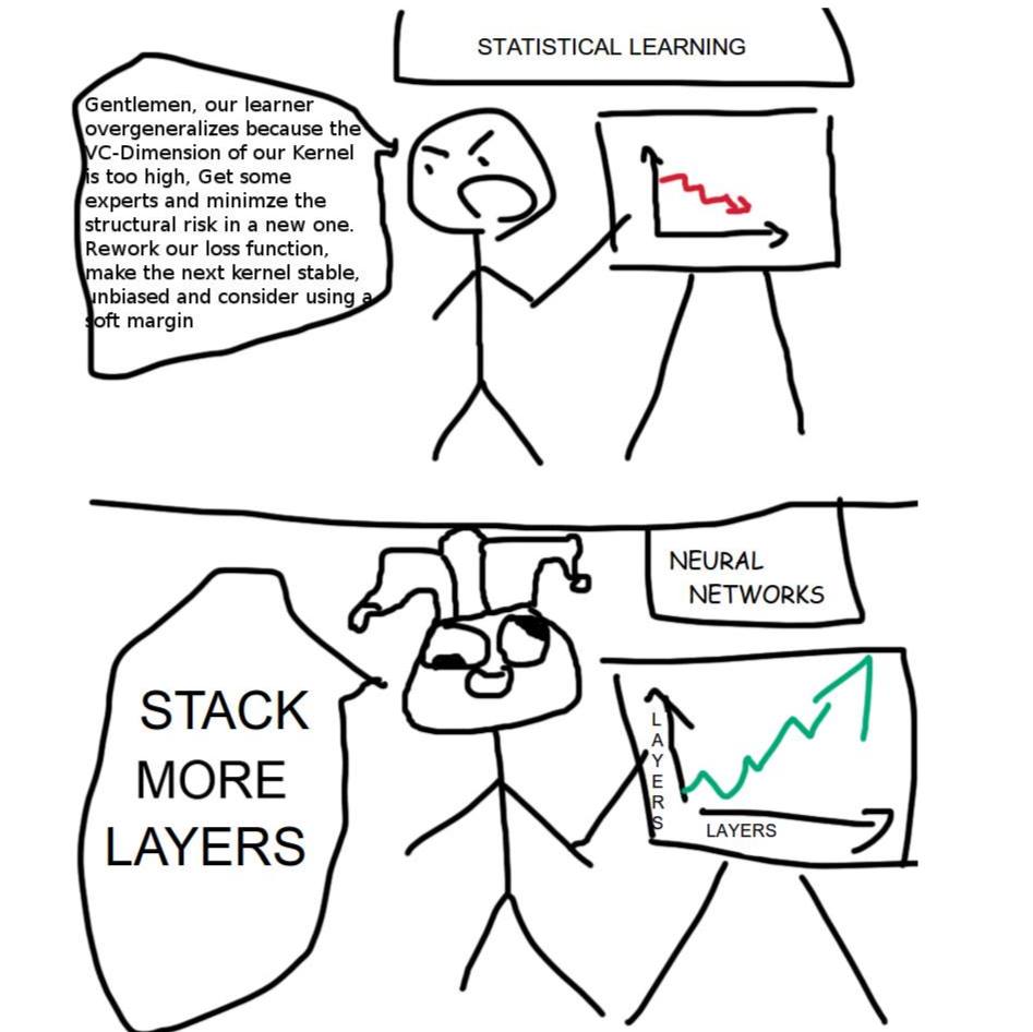] ] .kol-6-12[ ] ] --- count: false # Reputation of Deep Learning .grid[ .kol-6-12[ .center[] ] .kol-6-12[ - .Q[Why would it be a good idea to stack more layers?] - .Q[Are there any theoretical insights for doing his? Empirical ones?] ] ] --- # Outline ## Universal approximation theorem ## Why going deeper? ## Regularization in deep networks ### classic regularization: $L\_2$ regularization ### implicit regularization: Dropout, Batch Normalization ## Residual networks --- class: center, middle # Going deeper --- # Universal function approximation .bold[Theorem.] ( Hornik et al, 1991) Let $\sigma$ be a nonconstant, bounded, and monotonically-increasing continuous function. For any $f \in C([0, 1]^{d})$ and $\varepsilon > 0$, there exists $h \in \mathbb{N}$ real constants $v\_i, b\_i \in \mathbb{R}$ and real vectors $w_i \in \mathbb{R}^d$ such that: $$ | \sum\_i^h v\_i \sigma(w\_i^Tx + b\_i) - f (x) | < \varepsilon $$ that is: neural nets are dense in $C([0, 1]^{d})$. .credit[Slide credit: G. Louppe] .citation[K. Hornik et al., Approximation Capabilities of Multilayer Feedforward Networks, 1991] -- count: false - It guarantees that even a single hidden-layer network can represent any classification problem in which the boundary is locally linear (smooth); - It does not inform about good/bad architectures, nor how they relate to the optimization procedure. - The universal approximation theorem generalizes to any non-polynomial (possibly unbounded) activation function, including the ReLU (Leshno, 1993). --- .bold[Theorem] (Barron, 1992) The mean integrated square error between the estimated network $\hat{F}$ and the target function $f$ is bounded by $$O\left(\frac{C^2\_f}{q} + \frac{qp}{N}\log N\right)$$ where $N$ is the number of training points, $q$ is the number of neurons, $p$ is the input dimension, and $C\_f$ measures the global smoothness of $f$. .credit[Slide credit: G. Louppe] -- __.bold[tl;dr:]__ Provided enough data, it guarantees that adding more neurons will result in a better approximation. --- # Problem solved? UFA theorems **do not tell us**: - The number $h$ of hidden units small enough to have the network fit in RAM. - The optimal function parameters can be found in finite time by minimizing the Empirical Risk with SGD and the usual random initialization schemes. --- # Approximation with ReLU nets .left-column[ ```python import numpy as np import matplotlib.pyplot as plt def relu(x): return np.maximum(x, 0) def rect(x, a, b, h, eps=1e-7): return h / eps * ( relu(x - a) - relu(x - (a + eps)) - relu(x - b) + relu(x - (b + eps))) x = np.linspace(-3, 3, 1000) *y = ( rect(x, -1, 0, 0.4)) plt.plot(x, y) ``` ] .right-column[ <img src="images/part4/rectangle.svg" width="100%" /> ] .reset-columns[ ] .citation[Conner Davis, [Quora: Is a single layered ReLU network still a universal approximator?](https://www.quora.com/Is-a-single-layered-ReLu-network-still-a-universal-approximator)] --- # Approximation with ReLU nets .left-column[ ```python import numpy as np import matplotlib.pyplot as plt def relu(x): return np.maximum(x, 0) def rect(x, a, b, h, eps=1e-7): return h / eps * ( relu(x - a) - relu(x - (a + eps)) - relu(x - b) + relu(x - (b + eps))) x = np.linspace(-3, 3, 1000) *y = ( rect(x, -1, 0, 0.4) * + rect(x, 0, 1, 1.3) * + rect(x, 1, 2, 0.8)) plt.plot(x, y) ``` ] .right-column[ <img src="images/part4/many_rectangles_1.svg" width="100%" /> ] .reset-columns[ ] .citation[Conner Davis, [Quora: Is a single layered ReLU network still a universal approximator?](https://www.quora.com/Is-a-single-layered-ReLu-network-still-a-universal-approximator)] --- # Approximation with ReLU nets .left-column[ ```python import numpy as np import matplotlib.pyplot as plt def relu(x): return np.maximum(x, 0) def rect(x, a, b, h, eps=1e-7): return h / eps * ( relu(x - a) - relu(x - (a + eps)) - relu(x - b) + relu(x - (b + eps))) *x = np.arange(0,5,0.05) # 10 z = np.arange(0,5,0.001) sin_approx = np.zeros_like(z) *for i in range(2, x.size-1): * sin_approx = sin_approx + rect(z,(x[i]+x[i-1])/2, * (x[i]+x[i+1])/2, np.sin(x[i]), 1e-7) plt.plot(x, y) ``` ] .right-column[ <img src="images/part4/many_rectangles_2.svg" width="100%" /> ] .reset-columns[ ] .citation[Conner Davis, [Quora: Is a single layered ReLU network still a universal approximator?](https://www.quora.com/Is-a-single-layered-ReLu-network-still-a-universal-approximator)] --- # Approximation with ReLU nets .left-column[ ```python import numpy as np import matplotlib.pyplot as plt def relu(x): return np.maximum(x, 0) def rect(x, a, b, h, eps=1e-7): return h / eps * ( relu(x - a) - relu(x - (a + eps)) - relu(x - b) + relu(x - (b + eps))) *x = np.arange(0,5,0.25) # 20 z = np.arange(0,5,0.001) sin_approx = np.zeros_like(z) *for i in range(2, x.size-1): * sin_approx = sin_approx + rect(z,(x[i]+x[i-1])/2, * (x[i]+x[i+1])/2, np.sin(x[i]), 1e-7) plt.plot(x, y) ``` ] .right-column[ <img src="images/part4/many_rectangles_3.svg" width="100%" /> ] .reset-columns[ ] .citation[Conner Davis, [Quora: Is a single layered ReLU network still a universal approximator?](https://www.quora.com/Is-a-single-layered-ReLu-network-still-a-universal-approximator)] --- # Approximation with ReLU nets .left-column[ ```python import numpy as np import matplotlib.pyplot as plt def relu(x): return np.maximum(x, 0) def rect(x, a, b, h, eps=1e-7): return h / eps * ( relu(x - a) - relu(x - (a + eps)) - relu(x - b) + relu(x - (b + eps))) *x = np.arange(0,5,0.1) # 50 z = np.arange(0,5,0.001) sin_approx = np.zeros_like(z) *for i in range(2, x.size-1): * sin_approx = sin_approx + rect(z,(x[i]+x[i-1])/2, * (x[i]+x[i+1])/2, np.sin(x[i]), 1e-7) plt.plot(x, y) ``` ] .right-column[ <img src="images/part4/many_rectangles_4.svg" width="100%" /> ] .reset-columns[ ] .citation[Conner Davis, [Quora: Is a single layered ReLU network still a universal approximator?](https://www.quora.com/Is-a-single-layered-ReLu-network-still-a-universal-approximator)] --- # Approximation with ReLU nets .left-column[ ```python import numpy as np import matplotlib.pyplot as plt def relu(x): return np.maximum(x, 0) def rect(x, a, b, h, eps=1e-7): return h / eps * ( relu(x - a) - relu(x - (a + eps)) - relu(x - b) + relu(x - (b + eps))) *x = np.arange(0,5,0.01) # 500 z = np.arange(0,5,0.001) sin_approx = np.zeros_like(z) *for i in range(2, x.size-1): * sin_approx = sin_approx + rect(z,(x[i]+x[i-1])/2, * (x[i]+x[i+1])/2, np.sin(x[i]), 1e-7) plt.plot(x, y) ``` ] .right-column[ <img src="images/part4/many_rectangles_5.svg" width="100%" /> ] .reset-columns[ ] .citation[Conner Davis, [Quora: Is a single layered ReLU network still a universal approximator?](https://www.quora.com/Is-a-single-layered-ReLu-network-still-a-universal-approximator)] --- # Approximation with ReLU nets Consider the 1-layer MLP: $f(x) = \sum w\_i \text{ReLU}(x + b_i).$ <br/> This model can approximate any smooth 1D function with a linear combination of translated/scaled ReLU functions. $$f(x) = \sigma(w\_1 x + b_1)$$ .center[<img src="images/part4/ua-0.png">] .credit[Figure credit: G. Louppe] --- class: middle count: false Consider the 1-layer MLP: $f(x) = \sum w\_i \text{ReLU}(x + b_i).$ <br/> This model can approximate any smooth 1D function with a linear combination of translated/scaled ReLU functions. $$f(x) = \sigma(w\_1 x + b_1) + \sigma(w\_2 x + b_2)$$ .center[<img src="images/part4/ua-1.png">] .credit[Figure credit: G. Louppe] --- class: middle count: false Consider the 1-layer MLP: $f(x) = \sum w\_i \text{ReLU}(x + b_i).$ <br/> This model can approximate any smooth 1D function with a linear combination of translated/scaled ReLU functions. $$f(x) = \sigma(w\_1 x + b_1) + \sigma(w\_2 x + b_2) + \sigma(w\_3 x + b_3)$$ .center[<img src="images/part4/ua-2.png">] .credit[Figure credit: G. Louppe] --- class: middle count: false Consider the 1-layer MLP: $f(x) = \sum w\_i \text{ReLU}(x + b_i).$ <br/> This model can approximate any smooth 1D function with a linear combination of translated/scaled ReLU functions. $$f(x) = \sigma(w\_1 x + b_1) + \sigma(w\_2 x + b_2) + \sigma(w\_3 x + b_3) + \dots$$ .center[<img src="images/part4/ua-3.png">] .credit[Figure credit: G. Louppe] --- class: middle count: false Consider the 1-layer MLP: $f(x) = \sum w\_i \text{ReLU}(x + b_i).$ <br/> This model can approximate any smooth 1D function with a linear combination of translated/scaled ReLU functions. $$f(x) = \sigma(w\_1 x + b_1) + \sigma(w\_2 x + b_2) + \sigma(w\_3 x + b_3) + \dots$$ .center[<img src="images/part4/ua-4.png">] .credit[Figure credit: G. Louppe] --- class: middle count: false Consider the 1-layer MLP: $f(x) = \sum w\_i \text{ReLU}(x + b_i).$ <br/> This model can approximate any smooth 1D function with a linear combination of translated/scaled ReLU functions. $$f(x) = \sigma(w\_1 x + b_1) + \sigma(w\_2 x + b_2) + \sigma(w\_3 x + b_3) + \dots$$ .center[<img src="images/part4/ua-5.png">] .credit[Figure credit: G. Louppe] --- class: middle count: false Consider the 1-layer MLP: $f(x) = \sum w\_i \text{ReLU}(x + b_i).$ <br/> This model can approximate any smooth 1D function with a linear combination of translated/scaled ReLU functions. $$f(x) = \sigma(w\_1 x + b_1) + \sigma(w\_2 x + b_2) + \sigma(w\_3 x + b_3) + \dots$$ .center[<img src="images/part4/ua-6.png">] .credit[Figure credit: G. Louppe] --- class: middle count: false Consider the 1-layer MLP: $f(x) = \sum w\_i \text{ReLU}(x + b_i).$ <br/> This model can approximate any smooth 1D function with a linear combination of translated/scaled ReLU functions. $$f(x) = \sigma(w\_1 x + b_1) + \sigma(w\_2 x + b_2) + \sigma(w\_3 x + b_3) + \dots$$ .center[<img src="images/part4/ua-7.png">] .credit[Figure credit: G. Louppe] --- class: middle count: false Consider the 1-layer MLP: $f(x) = \sum w\_i \text{ReLU}(x + b_i).$ <br/> This model can approximate any smooth 1D function with a linear combination of translated/scaled ReLU functions. $$f(x) = \sigma(w\_1 x + b_1) + \sigma(w\_2 x + b_2) + \sigma(w\_3 x + b_3) + \dots$$ .center[<img src="images/part4/ua-8.png">] .credit[Figure credit: G. Louppe] --- class: middle count: false Consider the 1-layer MLP: $f(x) = \sum w\_i \text{ReLU}(x + b_i).$ <br/> This model can approximate any smooth 1D function with a linear combination of translated/scaled ReLU functions. $$f(x) = \sigma(w\_1 x + b_1) + \sigma(w\_2 x + b_2) + \sigma(w\_3 x + b_3) + \dots$$ .center[<img src="images/part4/ua-9.png">] .credit[Figure credit: G. Louppe] --- class: middle count: false Consider the 1-layer MLP: $f(x) = \sum w\_i \text{ReLU}(x + b_i).$ <br/> This model can approximate any smooth 1D function with a linear combination of translated/scaled ReLU functions. $$f(x) = \sigma(w\_1 x + b_1) + \sigma(w\_2 x + b_2) + \sigma(w\_3 x + b_3) + \dots$$ .center[<img src="images/part4/ua-10.png">] .credit[Figure credit: G. Louppe] --- class: middle count: false Consider the 1-layer MLP: $f(x) = \sum w\_i \text{ReLU}(x + b_i).$ <br/> This model can approximate any smooth 1D function with a linear combination of translated/scaled ReLU functions. $$f(x) = \sigma(w\_1 x + b_1) + \sigma(w\_2 x + b_2) + \sigma(w\_3 x + b_3) + \dots$$ .center[<img src="images/part4/ua-11.png">] .credit[Figure credit: G. Louppe] --- class: middle count: false Consider the 1-layer MLP: $f(x) = \sum w\_i \text{ReLU}(x + b_i).$ <br/> This model can approximate any smooth 1D function with a linear combination of translated/scaled ReLU functions. $$f(x) = \sigma(w\_1 x + b_1) + \sigma(w\_2 x + b_2) + \sigma(w\_3 x + b_3) + \dots$$ .center[<img src="images/part4/ua-12.png">] .credit[Figure credit: G. Louppe] --- # Universal approximation Even if the MLP is able to represent the function, learning can fail for two different reasons: - the optimization algorithm may not be able to find the value of the parameters that correspond to the desired function - the training algorithm might chose the wrong function as result of overfitting --- # Universal approximation .grid[ .kol-4-12[ .center[] ] .kol-4-12[ .center[] ] .kol-4-12[ .center[] ] ] --- # Universal approximation Adding more neurons .left-column[ .center.width-90[] ] .right-column[ .center.width-90[] ] --- # Overparametrization and optimization ## Folklore experiment .left-column[ .center.width-60[] _Step 1:_ Generate labeled data by feeding random input vectors into depth $2$ net with hidden layer of size $n$ ] .right-column[ .center.width-60[] _Step 2:_ Difficult to train a new network using this labeled data with the same amount of hidden nodes. ] .citation[Livni et al.; 2014] --- count:false # Overparametrization and optimization ## Folklore experiment .left-column[ .center.width-60[] _Step 1:_ Generate labeled data by feeding random input vectors into depth $2$ net with hidden layer of size $n$ ] .right-column[ .center.width-60[] _Step 2:_ Difficult to train a new network using this labeled data with the same amount of hidden nodes. .red[It is much easier to train a new net with bigger hidden layer or addition layer] ] .citation[Livni et al.; 2014] --- class: middle # Benefits of depth --- # The benefits of depth .caption[GINN: Geometric Illustrations for Neural Networks (http://www.bayeswatch.com/2018/09/17/GINN/)] .center.width-40[] --- # Efficient Oscillations with Composition .left-column[ ```python import numpy as np import matplotlib.pyplot as plt def relu(x): return np.maximum(x, 0) def tri(x): return relu( relu(2 * x) - relu(4 * x - 2)) x = np.linspace(-.3, 1.3, 1000) y = tri(x) plt.plot(x, y) ``` ] .right-column[ <img src="images/part4/triangle_x.svg" width="100%" /> ] .citation[M. Telgarsky, [Benefits of depth in neural networks](https://www.youtube.com/watch?v=ssaXJqG9Dz4), COLT 2016 ] --- # Efficient Oscillations with Composition .left-column[ ```python import numpy as np import matplotlib.pyplot as plt def relu(x): return np.maximum(x, 0) def tri(x): return relu( relu(2 * x) - relu(4 * x - 2)) x = np.linspace(-.3, 1.3, 1000) *y = tri(tri(x)) plt.plot(x, y) ``` ] .right-column[ <img src="images/part4/triangle_triangle_x.svg" width="100%" /> ] .citation[M. Telgarsky, [Benefits of depth in neural networks](https://www.youtube.com/watch?v=ssaXJqG9Dz4), COLT 2016 ] --- # Efficient Oscillations with Composition .left-column[ ```python import numpy as np import matplotlib.pyplot as plt def relu(x): return np.maximum(x, 0) def tri(x): return relu( relu(2 * x) - relu(4 * x - 2)) x = np.linspace(-.3, 1.3, 1000) *y = tri(tri(tri(x))) plt.plot(x, y) ``` ] .right-column[ <img src="images/part4/triangle_triangle_triangle_x.svg" width="100%" /> ] .center[ 1 more layer → 2x more oscillations ] .citation[M. Telgarsky, [Benefits of depth in neural networks](https://www.youtube.com/watch?v=ssaXJqG9Dz4), COLT 2016 ] --- # Efficient Oscillations with Composition .left-column[ ```python import numpy as np import matplotlib.pyplot as plt def relu(x): return np.maximum(x, 0) def tri(x): return relu( relu(2 * x) - relu(4 * x - 2)) x = np.linspace(-.3, 1.3, 1000) *y = tri(tri(tri(tri(x)))) plt.plot(x, y) ``` ] .right-column[ <img src="images/part4/triangle_triangle_triangle_triangle_x.svg" width="100%" /> ] .center[ 1 more layer → 2x more oscillations ] .citation[M. Telgarsky, [Benefits of depth in neural networks](https://www.youtube.com/watch?v=ssaXJqG9Dz4), COLT 2016 ] --- # Efficient Oscillations with Composition .left-column[ - Adding the parameters required for **one new layer** can **multiply by two the number of local oscillations** in the decision function of the model. - This is to be constrasted with the approach of adding parameters **on the same layer** (as in the rectangle example) that can only contribute an **additive number of new local oscillations**. ] .right-column[ <img src="images/part4/triangle_triangle_triangle_triangle_x.svg" width="100%" /> ] .citation[M. Telgarsky, [Benefits of depth in neural networks](https://www.youtube.com/watch?v=ssaXJqG9Dz4), COLT 2016 ] --- class: middle .center[For a fixed parameter budget deeper is better] .center[ <img src="images/part4/depth-2-vs-depth-1.png" style="width: 700px;" /><br/> ] .citation.tiny[Montufar et al.; On the number of linear regions of deep neural networks; 2014] --- class: middle # The problem with depth --- class: middle Although it was known that _deeper is better_, for decades training deep neural networks was highly challenging and unstable. Besides limited hardware and data there were a few algorithmic flaws that have been fixed/softened in the last decade. --- # Vanishing gradients Training deep MLPs with many layers has for long (pre-2011) been very difficult due to the **vanishing gradient** problem. - Small gradients slow down, and eventually block, stochastic gradient descent. - This results in a limited capacity of learning. .center.width-60[<img src="images/part4/vanishing-gradient.png">] .caption[Backpropagated gradients normalized histograms (Glorot and Bengio, 2010).<br> Gradients for layers far from the output vanish to zero. ] .citation[Glorot and Bengio, Understanding the difficulty of training deep feedforward neural networks; AISTAT 2010] --- Consider a simplified 3-layer MLP, with $x, w\_1, w\_2, w\_3 \in\mathbb{R}$, such that $$f(x; w\_1, w\_2, w\_3) = \sigma\left(w\_3\sigma\left( w\_2 \sigma\left( w\_1 x \right)\right)\right). $$ Under the hood, this would be evaluated as $$\begin{aligned} u\_1 &= w\_1 x \\\\ u\_2 &= \sigma(u\_1) \\\\ u\_3 &= w\_2 u\_2 \\\\ u\_4 &= \sigma(u\_3) \\\\ u\_5 &= w\_3 u\_4 \\\\ \hat{y} &= \sigma(u\_5) \end{aligned}$$ .credit[Slide credit: G. Louppe] -- count:false and its derivative $\frac{\text{d}\hat{y}}{\text{d}w\_1}$ as $$\begin{aligned}\frac{\text{d}\hat{y}}{\text{d}w\_1} &= \frac{\partial \hat{y}}{\partial u\_5} \frac{\partial u\_5}{\partial u\_4} \frac{\partial u\_4}{\partial u\_3} \frac{\partial u\_3}{\partial u\_2}\frac{\partial u\_2}{\partial u\_1}\frac{\partial u\_1}{\partial w\_1}\\\\ &= \frac{\partial \sigma(u\_5)}{\partial u\_5} w\_3 \frac{\partial \sigma(u\_3)}{\partial u\_3} w\_2 \frac{\partial \sigma(u\_1)}{\partial u\_1} x \end{aligned}$$ --- class: middle The derivative of the sigmoid activation function $\sigma$ is: .center[<img src="images/part4/activation-grad-sigmoid.png">] $$\frac{\text{d} \sigma}{\text{d} x}(x) = \sigma(x)(1-\sigma(x))$$ Notice that $0 \leq \frac{\text{d} \sigma}{\text{d} x}(x) \leq \frac{1}{4}$ for all $x$. .credit[Slide credit: G. Louppe] --- class: middle Assume that weights $w\_1, w\_2, w\_3$ are initialized randomly from a Gaussian with zero-mean and small variance, such that with high probability $-1 \leq w\_i \leq 1$. Then, $$\frac{\text{d}\hat{y}}{\text{d}w\_1} = \underbrace{\frac{\partial \sigma(u\_5)}{\partial u\_5}}\_{\leq \frac{1}{4}} \underbrace{w\_3}\_{\leq 1} \underbrace{\frac{\partial \sigma(u\_3)}{\partial u\_3}}\_{\leq \frac{1}{4}} \underbrace{w\_2}\_{\leq 1} \underbrace{\frac{\sigma(u\_1)}{\partial u\_1}}\_{\leq \frac{1}{4}} x$$ This implies that the gradient $\frac{\text{d}\hat{y}}{\text{d}w\_1}$ **exponentially** shrinks to zero as the number of layers in the network increases. Hence the vanishing gradient problem. - In general, bounded activation functions (sigmoid, tanh, etc) are prone to the vanishing gradient problem. - Note the importance of a proper initialization scheme. .credit[Slide credit: G. Louppe] --- # Rectified linear units Instead of the sigmoid activation function, modern neural networks are for most based on **rectified linear units** (ReLU) (Glorot et al, 2011): $$\text{ReLU}(x) = \max(0, x)$$ .center[<img src="images/part4/activation-relu.png">] .credit[Slide credit: G. Louppe] --- class: middle Note that the derivative of the ReLU function is $$\frac{\text{d}}{\text{d}x} \text{ReLU}(x) = \begin{cases} 0 &\text{if } x \leq 0 \\\\ 1 &\text{otherwise} \end{cases}$$ .center[<img src="images/part4/activation-grad-relu.png">] For $x=0$, the derivative is undefined. In practice, it is set to zero. .credit[Slide credit: G. Louppe] --- class: middle Therefore, $$\frac{\text{d}\hat{y}}{\text{d}w\_1} = \underbrace{\frac{\partial \sigma(u\_5)}{\partial u\_5}}\_{= 1} w\_3 \underbrace{\frac{\partial \sigma(u\_3)}{\partial u\_3}}\_{= 1} w\_2 \underbrace{\frac{\partial \sigma(u\_1)}{\partial u\_1}}\_{= 1} x$$ This **solves** the vanishing gradient problem, even for deep networks! (provided proper initialization) Note that: - The ReLU unit dies when its input is negative, which might block gradient descent. - This is actually a useful property to induce *sparsity*. - This issue can also be solved using **leaky** ReLUs, defined as $$\text{LeakyReLU}(x) = \max(\alpha x, x)$$ for a small $\alpha \in \mathbb{R}^+$ (e.g., $\alpha=0.1$). --- class: middle The steeper slope in the loss surface speeds up the training. .center.width-30[] .citation[A. Krizhevsky et al., ImageNet Classification with Deep Convolutional Neural Networks; NIPS 2012] --- # Other activation functions - Several $\text{ReLU}$-like alternatives have been proposed in recent years: $\text{PReLU}$, $\text{ELU}$, $\text{SeLU}$, $\text{SReLU}$ .center.width-50[] .citation[[Visualising Activation Functions in Neural Networks](https://dashee87.github.io/data%20science/deep%20learning/visualising-activation-functions-in-neural-networks/)] --- class: center, middle # Regularization --- # Under-fitting and over-fitting What if we consider a hypothesis space $\mathcal{F}$ in which candidate functions $f$ are either too "simple" or too "complex" with respect to the true data generating process? .center[] --- class: middle .center.width-40[] Our goal is to find a function $f$ that makes good predictions on average from given data. We can consider $f$ as a polynomial of degree $D$ defined through its parameters $\mathbf{w} \in \mathbb{R}^D$ such that $$\hat{y} = f(x; \mathbf{w}) = \sum\_{d=0}^D w\_d x^d$$ --- class: middle count: false .center.width-60[] .credit[Slide credit: F. Fleuret] --- class: middle count: false .center.width-60[] .credit[Slide credit: F. Fleuret] --- class: middle count: false .center.width-60[] .credit[Slide credit: F. Fleuret] --- class: middle count: false .center.width-60[] .credit[Slide credit: F. Fleuret] --- class: middle count: false .center.width-60[] .credit[Slide credit: F. Fleuret] --- class: middle count: false .center.width-60[] .credit[Slide credit: F. Fleuret] --- class: middle count: false .center.width-60[] .credit[Slide credit: F. Fleuret] --- class: middle count: false .center.width-60[] .credit[Slide credit: F. Fleuret] --- class: middle count: false .center.width-60[] .credit[Slide credit: F. Fleuret] --- class: middle count: false .center.width-60[] .credit[Slide credit: F. Fleuret] --- class: middle .center.width-60[] .credit[Slide credit: F. Fleuret] --- class: middle Although it is difficult to define precisely, it is quite clear in practice how to increase or decrease it for a given class of models. For example: - The degree of polynomials; - The number of layers in a neural network; - The number of training iterations; - Regularization terms. --- class: middle # Regularization --- .center.width-100[] --- # Regularization We can reformulate the previously used squared error loss $$\ell(y, f(x;\mathbf{w})) = (y - f(x;\mathbf{w}))^2$$ to $$\ell(y, f(x;\mathbf{w})) = (y - f(x;\mathbf{w}))^2 + \rho \sum_{d}^{D} w\_d^2$$ <br> .Q.big.center[What will happen now?] --- # Regularization We can reformulate the previously used squared error loss $$\ell(y, f(x;\mathbf{w})) = (y - f(x;\mathbf{w}))^2$$ to $$\ell(y, f(x;\mathbf{w})) = (y - f(x;\mathbf{w}))^2 + \rho \sum_{d}^{D} w\_d^2$$ <br> .center.big[This is called __$L\_2$ regularization__.] --- class: middle .center.width-60[] .credit[Slide credit: F. Fleuret] --- class: middle count: false .center.width-60[] .credit[Slide credit: F. Fleuret] --- class: middle count: false .center.width-60[] .credit[Slide credit: F. Fleuret] --- class: middle count: false .center.width-60[] .credit[Slide credit: F. Fleuret] --- class: middle count: false .center.width-60[] .credit[Slide credit: F. Fleuret] --- class: middle count: false .center.width-60[] .credit[Slide credit: F. Fleuret] --- class: middle count: false .center.width-60[] .credit[Slide credit: F. Fleuret] --- class: middle count: false .center.width-60[] .credit[Slide credit: F. Fleuret] --- class: middle count: false .center.width-60[] .credit[Slide credit: F. Fleuret] --- class: middle count: false .center.width-60[] .credit[Slide credit: F. Fleuret] --- class: middle count: false .center.width-60[] .credit[Slide credit: F. Fleuret] --- class: middle count: false .center.width-60[] .credit[Slide credit: F. Fleuret] --- class: middle count: false .center.width-60[] .credit[Slide credit: F. Fleuret] --- class: middle count: false .center.width-60[] .credit[Slide credit: F. Fleuret] --- class: middle count: false .center.width-60[] .credit[Slide credit: F. Fleuret] --- class: middle count: false .center.width-60[] .credit[Slide credit: F. Fleuret] --- class: middle count: false .center.width-60[] .credit[Slide credit: F. Fleuret] --- # $L\_2$ regularization - in Deep Learning it is ofter referred to as __weight decay__ ```py torch.optim.SGD(params, lr=<required parameter>, momentum=0, dampening=0, weight_decay=0, nesterov=False) ``` ```py torch.optim.Adam(params, lr=0.001, betas=(0.9, 0.999), eps=1e-08, weight_decay=0, amsgrad=False) ``` --- class: center, middle # Deep regularization --- class: middle .width-40[] .citation[C. Zhang et al., Understanding deep learning requires rethinking generalization, ICLR 2017] --- count: false class: middle However ... .center.width-100[] .citation[C. Zhang et al., Understanding deep learning requires rethinking generalization, ICLR 2017] --- class: middle However ... .center.width-60[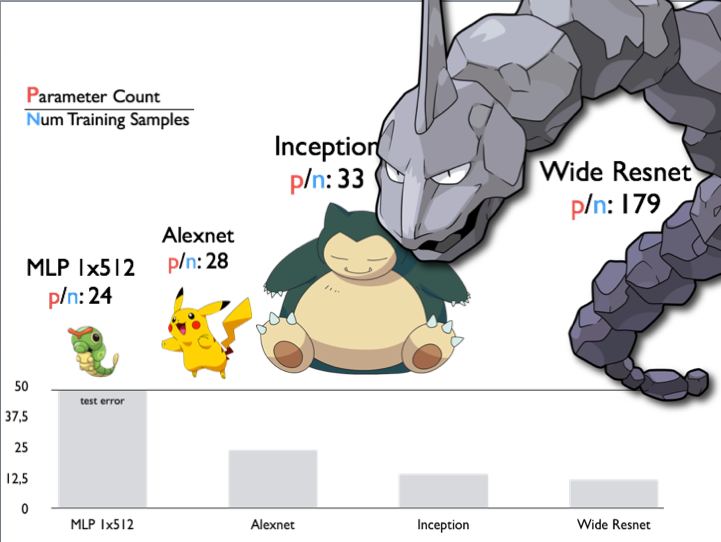] .citation[C. Zhang et al., Understanding deep learning requires rethinking generalization, ICLR 2017] --- class: middle, center ### Most of the weights of the network are grouped in the final layers. .center.width-80[] --- # VGG-16 .center[ <img src="images/part4/vgg.png" style="width: 600px;" /> ] .citation[K. Simonyan and A. Zisserman, Very deep convolutional networks for large-scale image recognition, NIPS 2014] --- # Memory and Parameters ```md Activation maps Parameters INPUT: [224x224x3] = 150K 0 CONV3-64: [224x224x64] = 3.2M (3x3x3)x64 = 1,728 CONV3-64: [224x224x64] = 3.2M (3x3x64)x64 = 36,864 POOL2: [112x112x64] = 800K 0 CONV3-128: [112x112x128] = 1.6M (3x3x64)x128 = 73,728 CONV3-128: [112x112x128] = 1.6M (3x3x128)x128 = 147,456 POOL2: [56x56x128] = 400K 0 CONV3-256: [56x56x256] = 800K (3x3x128)x256 = 294,912 CONV3-256: [56x56x256] = 800K (3x3x256)x256 = 589,824 CONV3-256: [56x56x256] = 800K (3x3x256)x256 = 589,824 POOL2: [28x28x256] = 200K 0 CONV3-512: [28x28x512] = 400K (3x3x256)x512 = 1,179,648 CONV3-512: [28x28x512] = 400K (3x3x512)x512 = 2,359,296 CONV3-512: [28x28x512] = 400K (3x3x512)x512 = 2,359,296 POOL2: [14x14x512] = 100K 0 CONV3-512: [14x14x512] = 100K (3x3x512)x512 = 2,359,296 CONV3-512: [14x14x512] = 100K (3x3x512)x512 = 2,359,296 CONV3-512: [14x14x512] = 100K (3x3x512)x512 = 2,359,296 POOL2: [7x7x512] = 25K 0 FC: [1x1x4096] = 4096 7x7x512x4096 = 102,760,448 FC: [1x1x4096] = 4096 4096x4096 = 16,777,216 FC: [1x1x1000] = 1000 4096x1000 = 4,096,000 TOTAL activations: 24M x 4 bytes ~= 93MB / image (x2 for backward) TOTAL parameters: 138M x 4 bytes ~= 552MB (x2 for plain SGD, x4 for Adam) ``` .credit[Slide credit: C. Ollion & O. Grisel] --- # Memory and Parameters ```md Activation maps Parameters INPUT: [224x224x3] = 150K 0 *CONV3-64: [224x224x64] = 3.2M (3x3x3)x64 = 1,728 *CONV3-64: [224x224x64] = 3.2M (3x3x64)x64 = 36,864 POOL2: [112x112x64] = 800K 0 CONV3-128: [112x112x128] = 1.6M (3x3x64)x128 = 73,728 CONV3-128: [112x112x128] = 1.6M (3x3x128)x128 = 147,456 POOL2: [56x56x128] = 400K 0 CONV3-256: [56x56x256] = 800K (3x3x128)x256 = 294,912 CONV3-256: [56x56x256] = 800K (3x3x256)x256 = 589,824 CONV3-256: [56x56x256] = 800K (3x3x256)x256 = 589,824 POOL2: [28x28x256] = 200K 0 CONV3-512: [28x28x512] = 400K (3x3x256)x512 = 1,179,648 CONV3-512: [28x28x512] = 400K (3x3x512)x512 = 2,359,296 CONV3-512: [28x28x512] = 400K (3x3x512)x512 = 2,359,296 POOL2: [14x14x512] = 100K 0 CONV3-512: [14x14x512] = 100K (3x3x512)x512 = 2,359,296 CONV3-512: [14x14x512] = 100K (3x3x512)x512 = 2,359,296 CONV3-512: [14x14x512] = 100K (3x3x512)x512 = 2,359,296 POOL2: [7x7x512] = 25K 0 *FC: [1x1x4096] = 4096 7x7x512x4096 = 102,760,448 FC: [1x1x4096] = 4096 4096x4096 = 16,777,216 FC: [1x1x1000] = 1000 4096x1000 = 4,096,000 TOTAL activations: 24M x 4 bytes ~= 93MB / image (x2 for backward) TOTAL parameters: 138M x 4 bytes ~= 552MB (x2 for plain SGD, x4 for Adam) ``` .credit[Slide credit: C. Ollion & O. Grisel] --- class: middle # Dropout --- # Dropout - First "deep" regularization technique - Remove units at random during the forward pass on each sample - Put them all back during test .center[ <img src="images/part4/dropout.png" style="width: 680px;" /> ] .citation[Srivastava et al., Dropout: A Simple Way to Prevent Neural Networks from Overfitting, JMLR 2014] --- # Dropout ## Interpretation - Reduces the network dependency to individual neurons and distributes representation - More redundant representation of data ## Ensemble interpretation - Equivalent to training a large ensemble of shared-parameters, binary-masked models - Each model is only trained on a single data point - __A network with dropout can be interpreted as an ensemble of $2^N$ models with heavy weight sharing__ (Goodfellow et al., 2013) --- # Dropout .center[ <img src="images/part4/dropout_traintest.png" style="width: 600px;" /><br/> ] - One has to decide on which units/layers to use dropout, and with what probability $p$ units are dropped. - During training, for each sample, as many Bernoulli variables as units are sampled independently to select units to remove. - To keep the means of the inputs to layers unchanged, the initial version of dropout was multiplying activations by $p$ during test. - The standard variant is the "inverted dropout": multiply activations by $\frac{1}{1-p}$ during training and keep the network untouched during test. --- # Dropout Overfitting noise .center[<img src="images/part4/dropout_curves_1.svg" style="width: 600px;" /><br/> ] .credit[Slide credit: C. Ollion & O. Grisel] --- count: false # Dropout A bit of Dropout .center[<img src="images/part4/dropout_curves_2.svg" style="width: 600px;" /><br/> ] .credit[Slide credit: C. Ollion & O. Grisel] --- count: false # Dropout Too much: underfitting .center[<img src="images/part4/dropout_curves_3.svg" style="width: 600px;" /><br/> ] .credit[Slide credit: C. Ollion & O. Grisel] --- count: false # Dropout .center.width-40[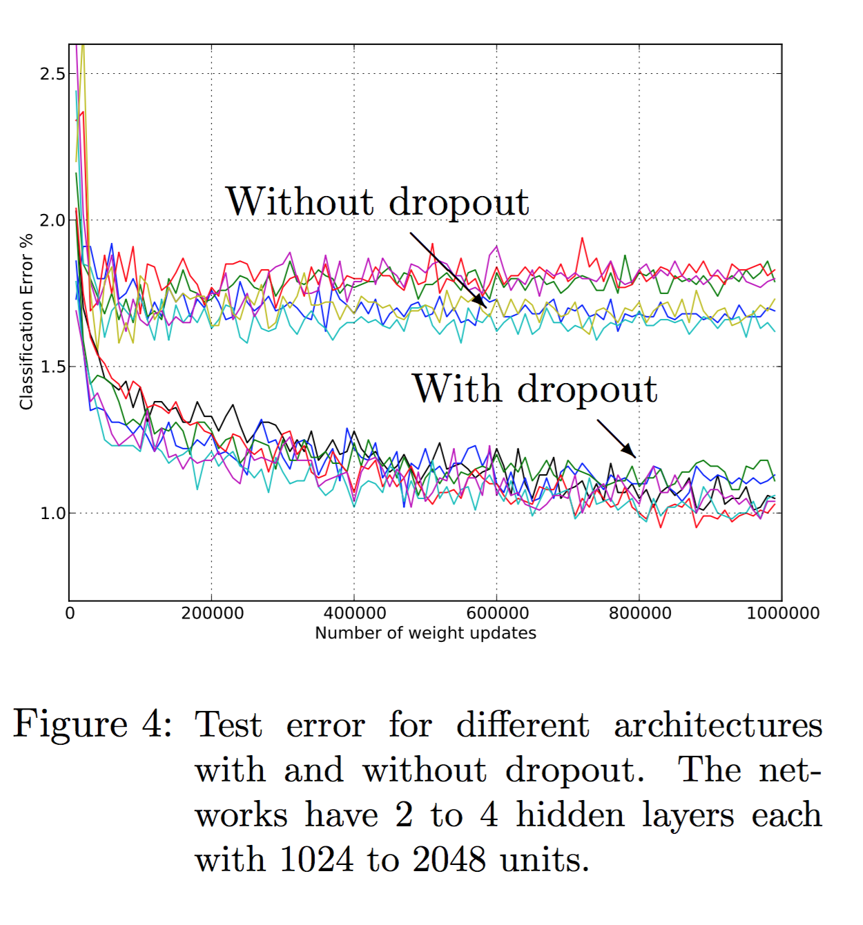] .citation[Srivastava et al., Dropout: A Simple Way to Prevent Neural Networks from Overfitting, JMLR 2014] --- # Dropout ```py >>> x = torch.full((3, 5), 1.0).requires_grad_() >>> x tensor([[ 1., 1., 1., 1., 1.], [ 1., 1., 1., 1., 1.], [ 1., 1., 1., 1., 1.]]) >>> dropout = nn.Dropout(p = 0.75) >>> y = dropout(x) >>> y tensor([[ 0., 0., 4., 0., 4.], [ 0., 4., 4., 4., 0.], [ 0., 0., 4., 0., 0.]]) >>> l = y.norm(2, 1).sum() >>> l.backward() >>> x.grad tensor([[ 0.0000, 0.0000, 2.8284, 0.0000, 2.8284] [ 0.0000, 2.3094, 2.3094, 2.3094, 0.0000] [ 0.0000, 0.0000, 4.0000, 0.0000, 0.0000]]) ``` --- count: false # Dropout ```py >>> x = torch.full((3, 5), 1.0).requires_grad_() >>> x tensor([[ 1., 1., 1., 1., 1.], [ 1., 1., 1., 1., 1.], [ 1., 1., 1., 1., 1.]]) >>> dropout = nn.Dropout(p = 0.75) >>> y = dropout(x) *>>> y *tensor([[ 0., 0., 4., 0., 4.], * [ 0., 4., 4., 4., 0.], * [ 0., 0., 4., 0., 0.]]) >>> l = y.norm(2, 1).sum() >>> l.backward() >>> x.grad tensor([[ 0.0000, 0.0000, 2.8284, 0.0000, 2.8284] [ 0.0000, 2.3094, 2.3094, 2.3094, 0.0000] [ 0.0000, 0.0000, 4.0000, 0.0000, 0.0000]]) ``` --- # Dropout For a given network ```py model = nn.Sequential(nn.Linear(10, 100), nn.ReLU(), nn.Linear(100, 50), nn.ReLU(), nn.Linear(50, 2)); ``` -- count: false we can simply add dropout layers ```py model = nn.Sequential(nn.Linear(10, 100), nn.ReLU(), * nn.Dropout(), nn.Linear(100, 50), nn.ReLU(), * nn.Dropout(), nn.Linear(50, 2)); ``` --- # Dropout A model using dropout has to be set in __train__ or __test__ mode --- count: false # Dropout A model using dropout has to be set in __train__ or __test__ mode The method `nn.Module.train(mode)` recursively sets the flag `training` to all sub-modules. ```py >>> dropout = nn.Dropout() >>> model = nn.Sequential(nn.Linear(3, 10), dropout, nn.Linear(10, 3)) >>> dropout.training True >>> model.train(False) Sequential ( (0): Linear (3 -> 10) (1): Dropout (p = 0.5) (2): Linear (10 -> 3) ) >>> dropout.training False ``` --- # Dropout A model using dropout has to be set in __train__ or __test__ mode ```py >>> dropout = nn.Dropout() >>> model = nn.Sequential(nn.Linear(3, 10), dropout, nn.Linear(10, 3)) >>> x = torch.full((1, 3), 1.0) *>>> model.train() Sequential ( (0): Linear (3 -> 10) (1): Dropout (p = 0.5) (2): Linear (10 -> 3) ) >>> model(x) *tensor([[ 0.5360, -0.5225, -0.5129]], grad_fn=<ThAddmmBackward>) >>> model(x) *tensor([[ 0.6134, -0.6130, -0.5161]], grad_fn=<ThAddmmBackward>) ``` --- count: false # Dropout A model using dropout has to be set in __train__ or __test__ mode ```py >>> dropout = nn.Dropout() >>> model = nn.Sequential(nn.Linear(3, 10), dropout, nn.Linear(10, 3)) >>> x = torch.full((1, 3), 1.0) >>> model.train() Sequential ( (0): Linear (3 -> 10) (1): Dropout (p = 0.5) (2): Linear (10 -> 3) ) >>> model(x) tensor([[ 0.5360, -0.5225, -0.5129]], grad_fn=<ThAddmmBackward>) >>> model(x) tensor([[ 0.6134, -0.6130, -0.5161]], grad_fn=<ThAddmmBackward>) >>> *>>> model.eval() Sequential ( (0): Linear (3 -> 10) (1): Dropout (p = 0.5) (2): Linear (10 -> 3) ) >>> model(x) *tensor([[ 0.5772, -0.0944, -0.1168]], grad_fn=<ThAddmmBackward>) >>> model(x) *tensor([[ 0.5772, -0.0944, -0.1168]], grad_fn=<ThAddmmBackward>) ``` --- # Spatial Dropout .grid[ .kol-6-12[ - The original Dropout is less compatible with convolutional layers. - Units in a 2d activation map are generally locally correlated, and dropout has virtually no effect. - An alternative is to drop channels instead of individual units. ] .kol-6-12[ ] ] --- count: false # Spatial Dropout .grid[ .kol-6-12[ - The original Dropout is less compatible with convolutional layers. - Units in a 2d activation map are generally locally correlated, and dropout has virtually no effect. - An alternative is to drop channels instead of individual units. ] .kol-6-12[ ```py >>> dropout2d = nn.Dropout2d() >>> x = Variable(Tensor(2, 3, 2, 2).fill_(1.0)) >>> dropout2d(x) Variable containing: (0 ,0 ,.,.) = 0 0 0 0 (0 ,1 ,.,.) = 0 0 0 0 (0 ,2 ,.,.) = 2 2 2 2 (1 ,0 ,.,.) = 2 2 2 2 (1 ,1 ,.,.) = 0 0 0 0 (1 ,2 ,.,.) = 2 2 2 2 [torch.FloatTensor of size 2x3x2x2] ``` ] ] --- #DropBlock .center.width-70[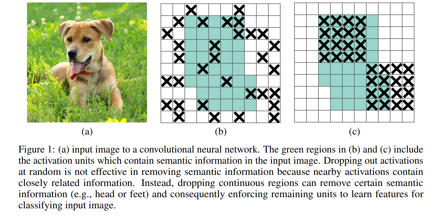] .center[Masking out continous regions in feature maps] .citation[G. Ghiasi et al.,DropBlock: A regularization method for convolutional networks, NIPS 2018] --- # Gaussian Dropout - we can generalize Bernoulli sampling over neurons, to sampling from other distributions - mutliplying activations and feature maps by a random variable drawn from $\mathcal{N}(1,1)$ works just as well, or perhaps bettern than using Bernoulli noise - this new form of dropout amounts to adding a Gaussian distributed random variable with zero mean and standard deviation equal to the activation of the unit - each hidden activation $h\_i$ is perturbed to: .center[$h\_i+h\_i r$ where $r \sim \mathcal{N}(0,1)$] or .center[$h\_i r'$ where $r' \sim \mathcal{N}(1,1)$] - we can generalize this to $r' \sim \mathcal{N}(1,\sigma^2)$, where $\sigma$ becomes and additional hyperparameter to tune, just like $p$ in standard Bernoulli dropout .citation[Srivastava et al., Dropout: A Simple Way to Prevent Neural Networks from Overfitting, JMLR 2014] --- class: middle # Batch Normalization --- # Batch normalization We saw that maintaining proper statistics of the activations and derivatives was a critical issue to allow the training of deep architectures. It is the main motivation behind weight initialization rules (we'll cover them later). --- count: false # Batch normalization We saw that maintaining proper statistics of the activations and derivatives was a critical issue to allow the training of deep architectures. It is the main motivation behind weight initialization rules (we'll cover them later). A different approach consists of explicitly forcing the activation statistics during the forward pass by re-normalizing them. __Batch normalization__ proposed by Ioffe and Szegedy (2015) was the first method introducing this idea. --- <br/><br/><br/><br/> "Training Deep Neural Networks is complicated by the fact that the __distribution of each layer's inputs changes during training, as the parameters of the previous layers change__. This slows down the training by requiring lower learning rates and careful parameter initialization ..." .pull-right[(Ioffe and Szegedy, 2015)] .citation[S. Ioffe and C. Szegedy, Batch Normalization: Accelerating Deep Network Training by Reducing Internal Covariate Shift; arXiv 2015] --- count: false <br/><br/><br/><br/> "Training Deep Neural Networks is complicated by the fact that the __distribution of each layer's inputs changes during training, as the parameters of the previous layers change__. This slows down the training by requiring lower learning rates and careful parameter initialization ..." .pull-right[(Ioffe and Szegedy, 2015)] .reset-column[ ] .center.width-60[] .citation[S. Ioffe and C. Szegedy, Batch Normalization: Accelerating Deep Network Training by Reducing Internal Covariate Shift; arXiv 2015] --- <br/> Consider a simplified 3-layer MLP, with $x, w\_1, w\_2, w\_3 \in\mathbb{R}$, such that $$f(x; w\_1, w\_2, w\_3) = \sigma\left(w\_3\sigma\left( w\_2 \sigma\left( w\_1 x \right)\right)\right). $$ Under the hood, this would be evaluated as $$\begin{aligned} u\_1 &= w\_1 x \\\\ u\_2 &= \sigma(u\_1) \\\\ u\_3 &= w\_2 u\_2 \\\\ u\_4 &= \sigma(u\_3) \\\\ u\_5 &= w\_3 u\_4 \\\\ \hat{y} &= \sigma(u\_5) \end{aligned}$$ .citation[S. Ioffe and C. Szegedy, Batch Normalization: Accelerating Deep Network Training by Reducing Internal Covariate Shift; arXiv 2015] -- count: false Batch normalization can be done anywhere in a deep architecture, and forces the activations' first and second order moments, so that the following layers do not need to adapt to their drift. --- # Batch normalization Normalize activations in each **mini-batch** before activation function: **speeds up** and **stabilizes** training (less dependent on init) .citation[S. Ioffe and C. Szegedy, Batch Normalization: Accelerating Deep Network Training by Reducing Internal Covariate Shift; arXiv 2015] -- count: false .center.width-50[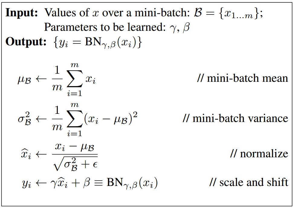] <br/> --- # Batch normalization During training batch normalization __shifts and rescales according to the mean and variance estimated on the batch__. .center.width-50[] <br/> .citation[S. Ioffe and C. Szegedy, Batch Normalization: Accelerating Deep Network Training by Reducing Internal Covariate Shift; arXiv 2015] --- # Batch normalization As for dropout, the model behaves differently during __train__ and __test__. At **test time**, use average and standard deviation computed on **the whole dataset** instead of batch Widely used in **ConvNets**, but requires the mini-batch to be large enough to compute statistics in the minibatch. --- # Batch normalization As dropout, batch normalization is implemented as a separate module `torch.BatchNorm1d` that processes the input components separately. ```py >>> x = torch.Tensor(10000, 3).normal_() >>> x = x * torch.Tensor([2., 5., 10.]) + torch.Tensor([-10., 25., 3.]) >>> x.mean(0) tensor([-9.9898, 24.9165,2.8945]) >>> x.std(0) tensor([2.0006, 5.0146, 9.9501]) >>> bn = nn.BatchNorm1d(3) >>> with torch.no_grad(): ... bn.bias.copy_(torch.tensor([2., 4., 8.])) ... bn.weight.copy_(torch.tensor([1., 2., 3.])) ... Parameter containing: tensor([2., 4., 8.]) Parameter containing: tensor([1., 2., 3.]) >>> y = bn(x) >>> y.mean(0) tensor([2.0000, 4.0000, 8.0000]) >>> y.std(0) tensor([1.0005, 2.0010, 3.0015]) ``` --- # Batch normalization `BatchNorm2d` example ```py >>> x = Variable(torch.randn(20, 100, 35, 45)) >>> bn2d = nn.BatchNorm2d(100) >>> y = bn2d(x) >>> x.size() torch.Size([20, 100, 35, 45]) >>> bn2d.weight.data.size() torch.Size([100]) >>> bn2d.bias.data.size() torch.Size([100]) ``` --- # Batch normalization Results on ImageNet LSVRC 2012: .center.width-70[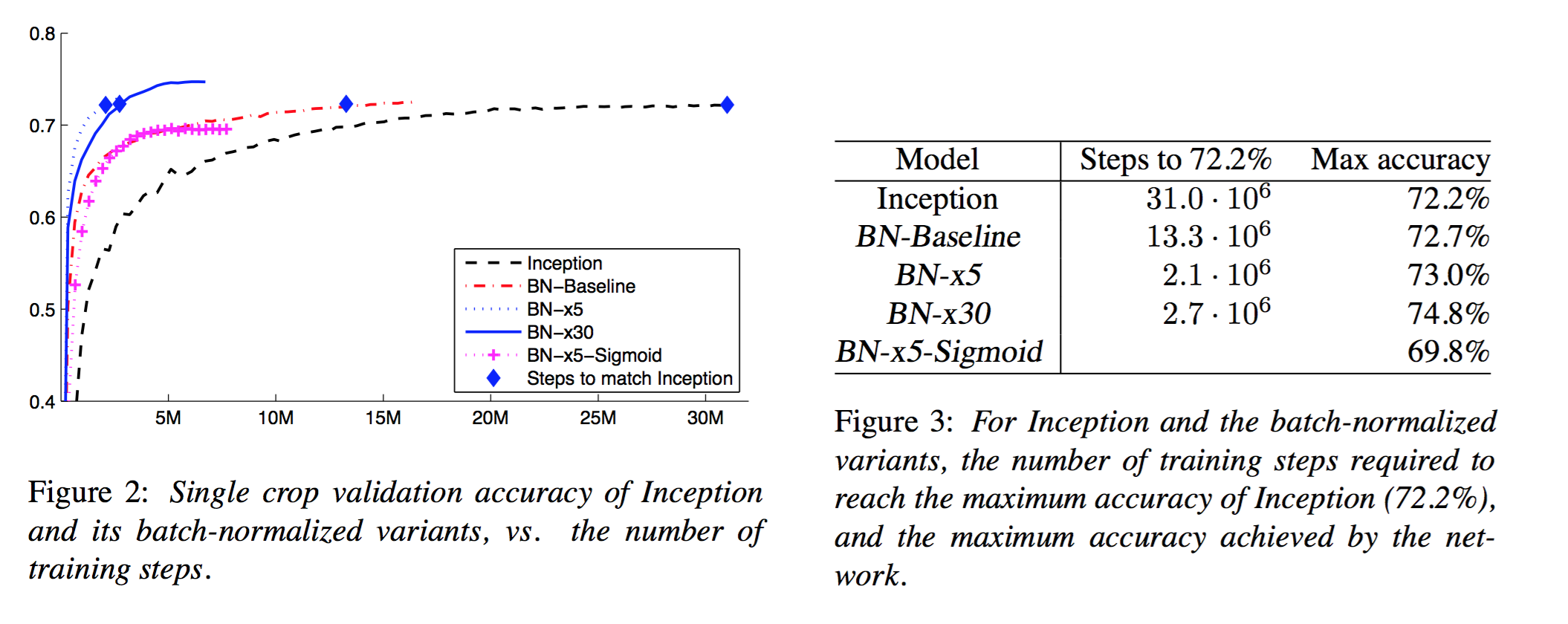] .citation[S. Ioffe and C. Szegedy, Batch Normalization: Accelerating Deep Network Training by Reducing Internal Covariate Shift; arXiv 2015] -- count: false - learning rate can be greater - dropout and local normalization are not necessary - $L^2$ regularization influence should be reduced --- The position of batch normalization relative to the non-linearity is not clear. .center.width-40[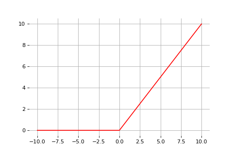 ] -- In the original paper, Ioffe and Szegedy, added BN right before nonlinearity: $$\dots \to \texttt{LINEAR} \to \texttt{BN} \to \texttt{ReLU} \to \dots$$ -- However, there are arguments for both ways: activations after the non-linearity are less "naturally normalized" and benefit more from batch normalization. Experiments are generally in favor of this solution, which is the current default. $$\dots \to \texttt{LINEAR} \to \texttt{ReLU} \to \texttt{BN} \to \dots$$ --- # Multiple variants <br> .center[ <img src="images/part4/cnn_normalizations.png" style="width: 800px;" /> ] .citation[Y. Wu and K. He, Group Normalization, ECCV 2018] --- class: middle # How deep can we go now? --- # A saturation point If we continue stacking more layers on a CNN: .center.width-90[] -- count: false .center[.red[Deeper models are harder to optimize]] --- .left-column[ # ResNet ] .right-column[ .center.width-50[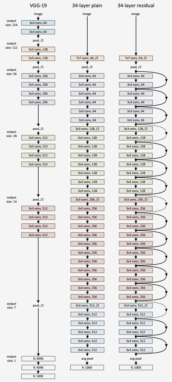] ] A block learns the residual w.r.t. identity .center.width-40[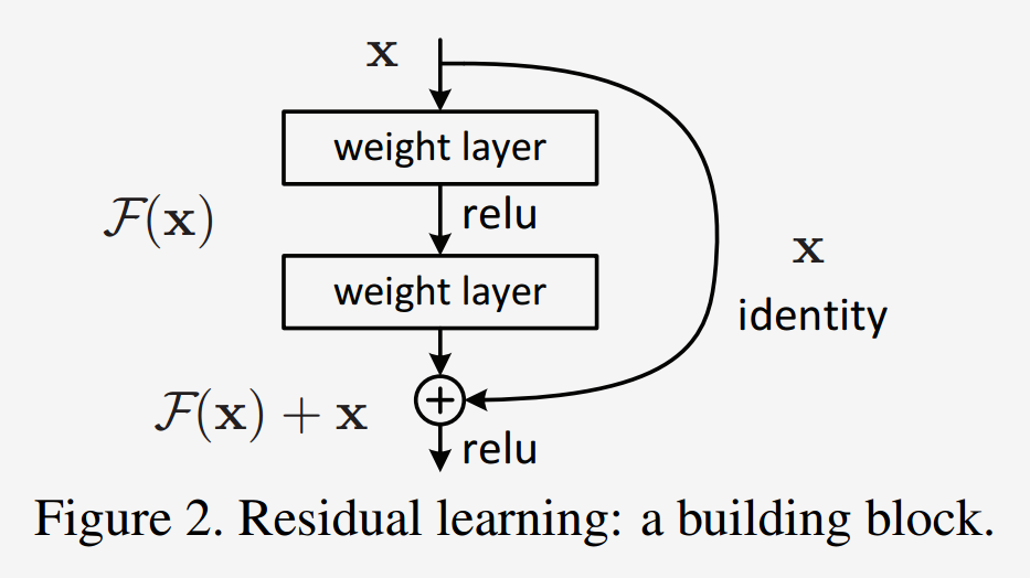] .citation[K. He et al., Deep residual learning for image recognition, CVPR 2016.] -- count: false - Good optimization properties --- .left-column[ # ResNet ] .right-column[ .center.width-50[] ] Even deeper models: 34, 50, 101, 152 layers .citation[K. He et al., Deep residual learning for image recognition, CVPR 2016.] --- .left-column[ # ResNet ] .right-column[ .center.width-50[] ] ResNet50 Compared to VGG: - Superior accuracy in all vision tasks <br/>**5.25%** top-5 error vs 7.1% .citation[K. He et al., Deep residual learning for image recognition, CVPR 2016.] -- count: false - Less parameters <br/>**25M** vs 138M -- count: false - Computational complexity <br/>**3.8B Flops** vs 15.3B Flops -- count: false - Fully Convolutional until the last layer --- # ResNet ## Performance on ImageNet .center.width-90[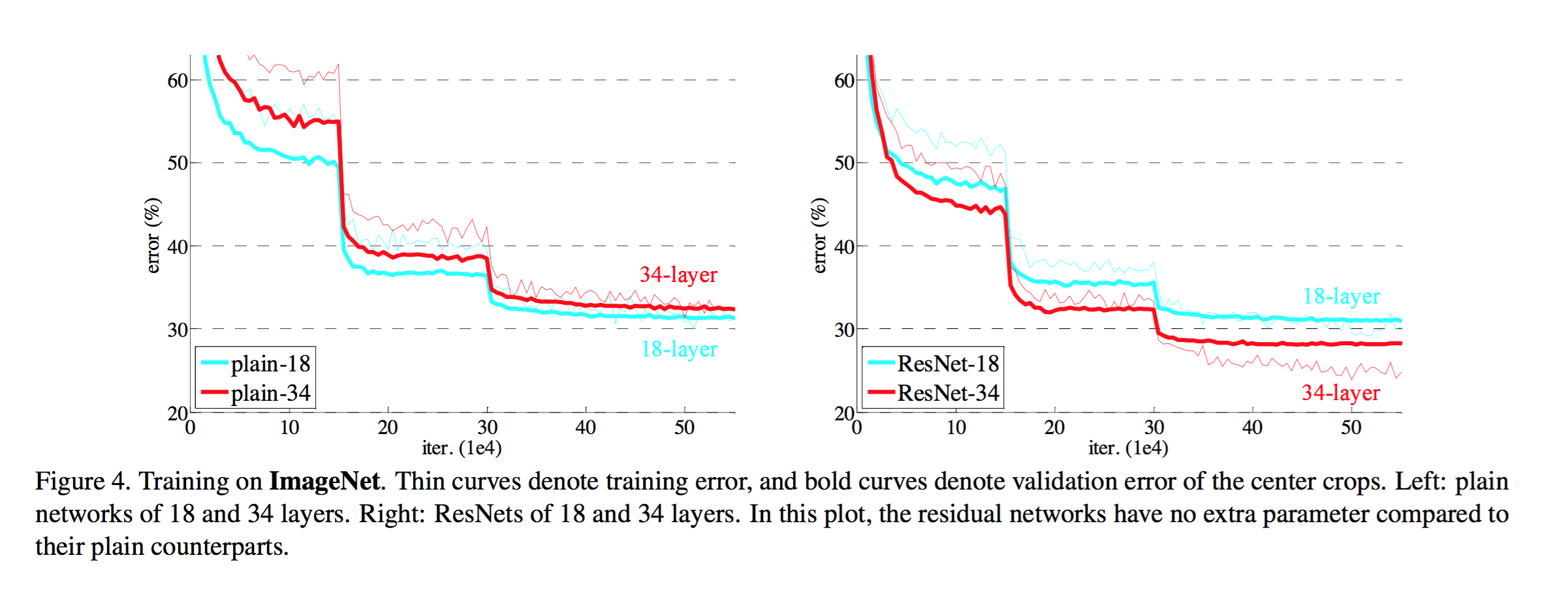] --- # ResNet ## Results .center.width-100[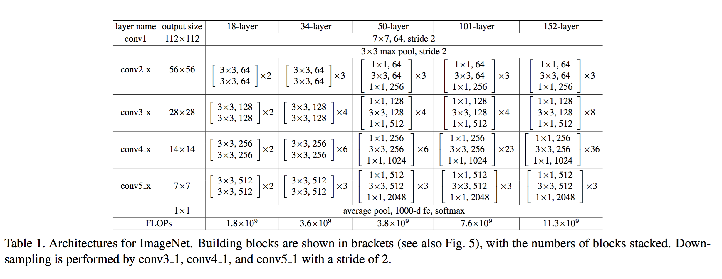] --- # ResNet ## Results .center.width-60[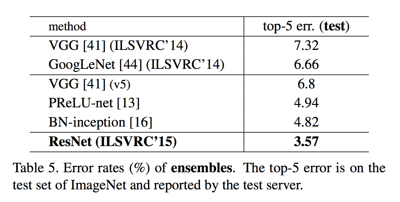] --- # ResNet In PyTorch: ```py def make_resnet_block(num_feature_maps , kernel_size = 3): return nn.Sequential( nn.Conv2d(num_feature_maps , num_feature_maps , kernel_size = kernel_size , padding = (kernel_size - 1) // 2), nn.BatchNorm2d(num_feature_maps), nn.ReLU(inplace = True), nn.Conv2d(num_feature_maps , num_feature_maps , kernel_size = kernel_size , padding = (kernel_size - 1) // 2), nn.BatchNorm2d(num_feature_maps), ) ``` --- # ResNet In PyTorch: ```py def __init__(self, num_residual_blocks, num_feature_maps) ... self.resnet_blocks = nn.ModuleList() for k in range(nb_residual_blocks): self.resnet_blocks.append(make_resnet_block(num_feature_maps , 3)) ... ``` ```py def forward(self,x): ... for b in self.resnet_blocks: * x = x + b(x) ... return x ``` --- For ResNet50+ layers some additional modifications need to be made to keep number of parameters and computations manageable .center.width-70[] Such a block requires $2 \times (3 \times 3 \times 256 +1) \times 256 \simeq 1.2M$ parameters .credit[Slide credit: F. Fleuret] -- count: false Adress this problem using __bottleneck__ block .center.width-100[] .center[$256 \times 64 + (3 \times 3 \times 64 +1) \times 64 + 64 \times 256 \simeq 70K$ parameters] --- # Stochastic Depth Networks - DropOut at layer level - Allows training up to 1K layers .center.width-70[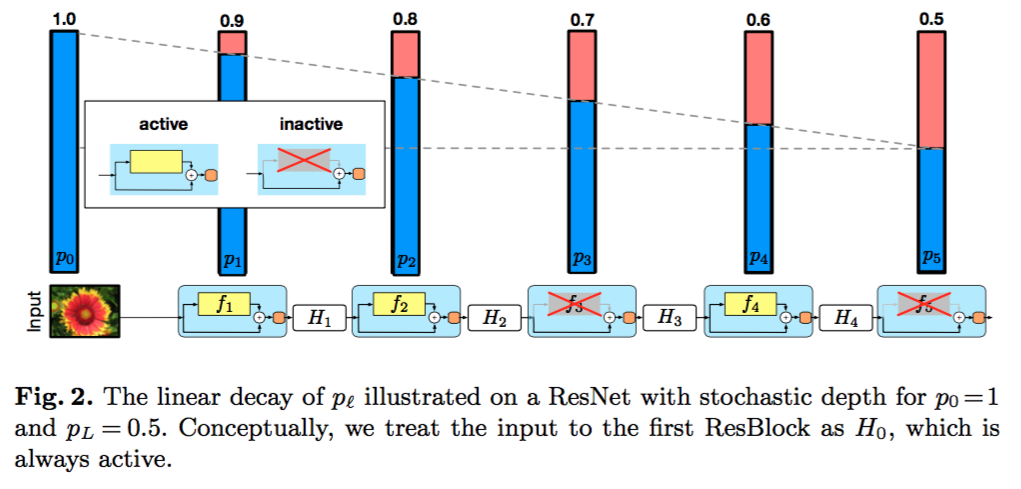] .citation[Huang et al., Deep Networks with Stochastic Depth, ECCV 2016] --- # DenseNet - Copying feature maps to upper layers via skip-connections - Better reuse of parameters and redundancy avoidance .center.width-30[] .center.width-70[] .citation[Huang et al., Densely Connected Convolutional Networks, CVPR 2017] --- # Visualizing loss surfaces .center.width-70[] .citation[H. Li et al., Visualizing the Loss Landscape of Neural Nets, ICLR workshop 2018] --- # Visualizing loss surfaces .left-column[ .center.width-100[] ] .right-column[ <br><br><br><br><br> - ResNet-20/56/110 : vanilla - ResNet-*-noshort: no skip connections - ResNet-18/34/50 : wide ] .citation[H. Li et al., Visualizing the Loss Landscape of Neural Nets, ICLR workshop 2018] --- # Visualizing loss surfaces .center.width-50[] .citation[H. Li et al., Visualizing the Loss Landscape of Neural Nets, ICLR workshop 2018] --- # Outline ## Universal approximation theorem ## Why going deeper? ## Regularization in deep networks ### classic regularization: $L\_2$ regularization ### implicit regularization: Dropout, Batch Normalization ## Residual networks --- class: end-slide, center count: false The end.