layout: true .center.footer[Marc LELARGE and Andrei BURSUC | Deep Learning Do It Yourself | 13. Siamese Networks] --- class: center, middle, title-slide count: false # 13. Siamese Networks and Representation Learning <br/> <br/> .bold[Andrei Bursuc ] <br/> url: https://dataflowr.github.io/website/ <!-- url: https://abursuc.github.io//slides/polytechnique/03_cnns_siamese.html --> .citation[ With slides from F. Fleuret, O. Grisel, E. Oyallon, G. Louppe, Y. Avrithis ...] --- # Siamese networks .center.width-60[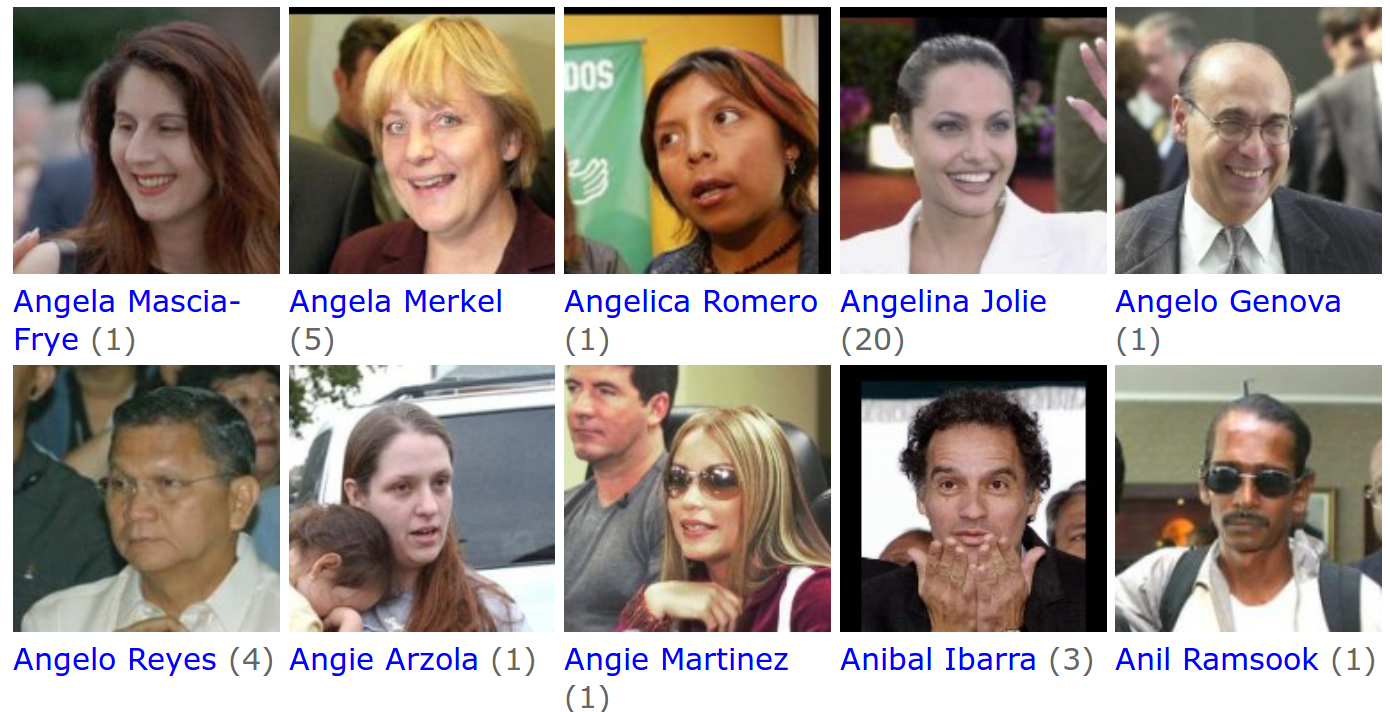] - **Recognition:** given a face, classify among K possible persons - **Verification:** verify that two faces belongs to the same person A verification system can be implemented as a similarity measure. If it's really good, useful for recognition. --- class: middle, center .big[Training a classifier with so many classes and so few samples per classes is challenging.] .hidden.big[In addition, for such use-cases, new classes can appear on the fly anytime.] --- count: false class: middle, center .big[Training a classifier with so many classes and so few samples per classes is challenging.] .big[In addition, for such use-cases, new classes can appear on the fly anytime.] --- class: middle, center .big[Instead of training a network to do classification, we can train it to compute useful features from images, allowing us to measure similarities/dissimilarities between images.] --- # Siamese architecture .center.width-60[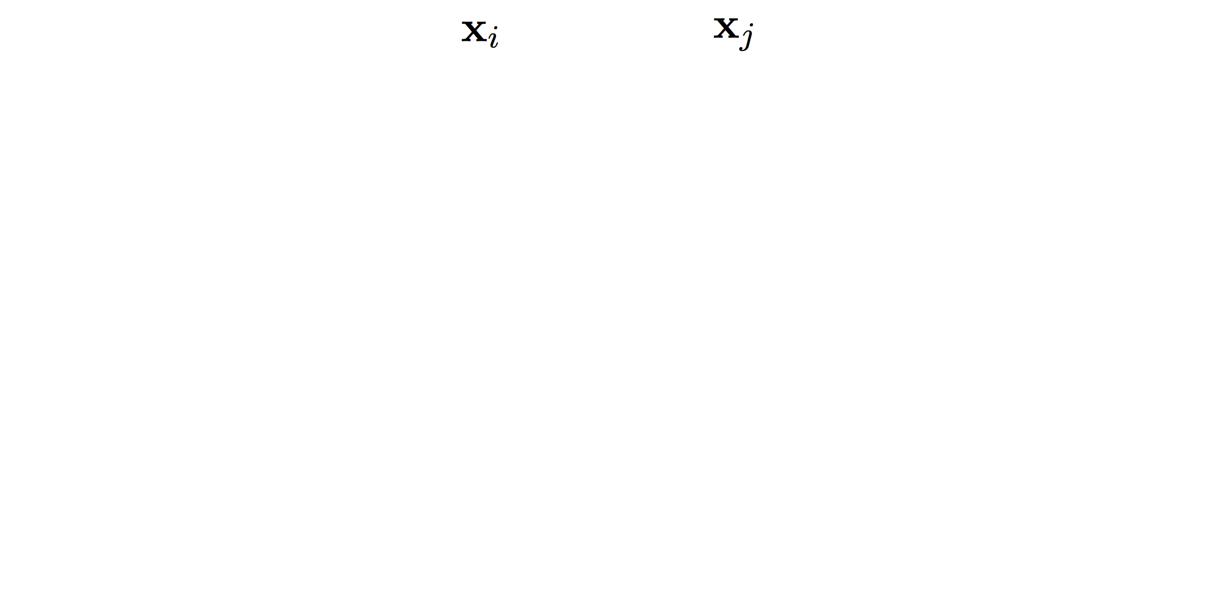] - an input sample is a _pair_ $( \mathbf{x}\_i, \mathbf{x}\_j)$ .citation[ S. Chopra et al.,Learning a similarity metric discriminatively, with application to face verification, CVPR 2005] --- # Siamese architecture .center.width-60[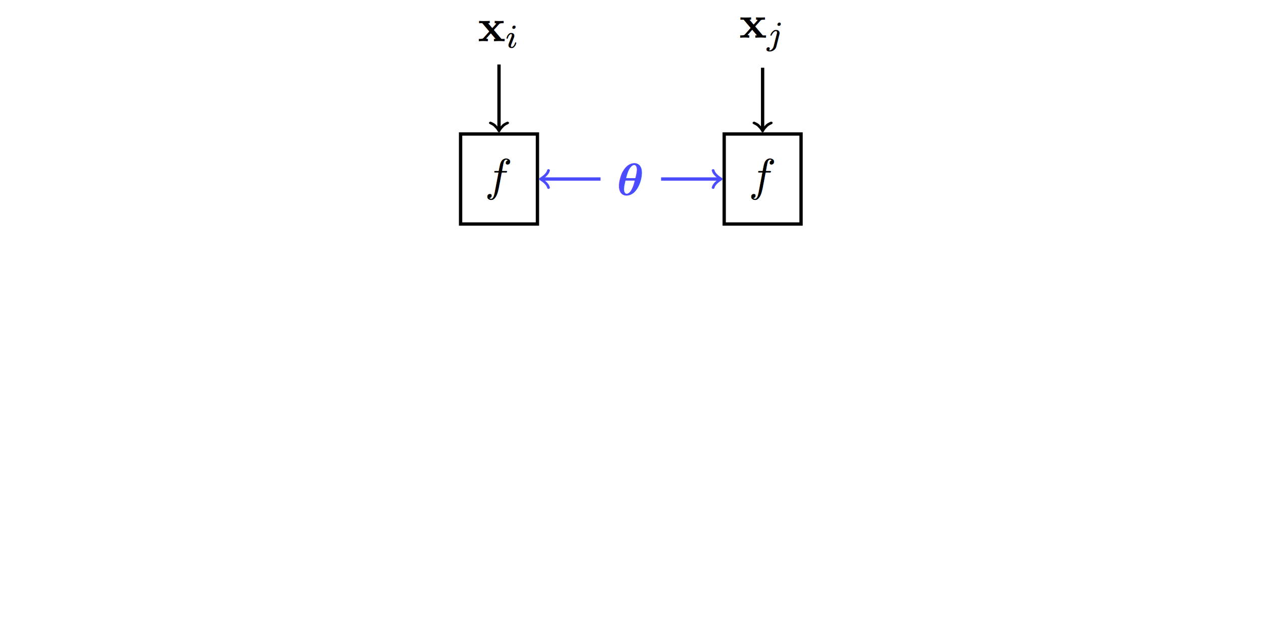] - an input sample is a _pair_ $( \mathbf{x}\_i, \mathbf{x}\_j)$ - both $\mathbf{x}\_i$, $\mathbf{x}\_j$ go through the _same_ function $f$ with _shared_ parameters $\theta$ .citation[ S. Chopra et al.,Learning a similarity metric discriminatively, with application to face verification, CVPR 2005] --- # Siamese architecture .center.width-60[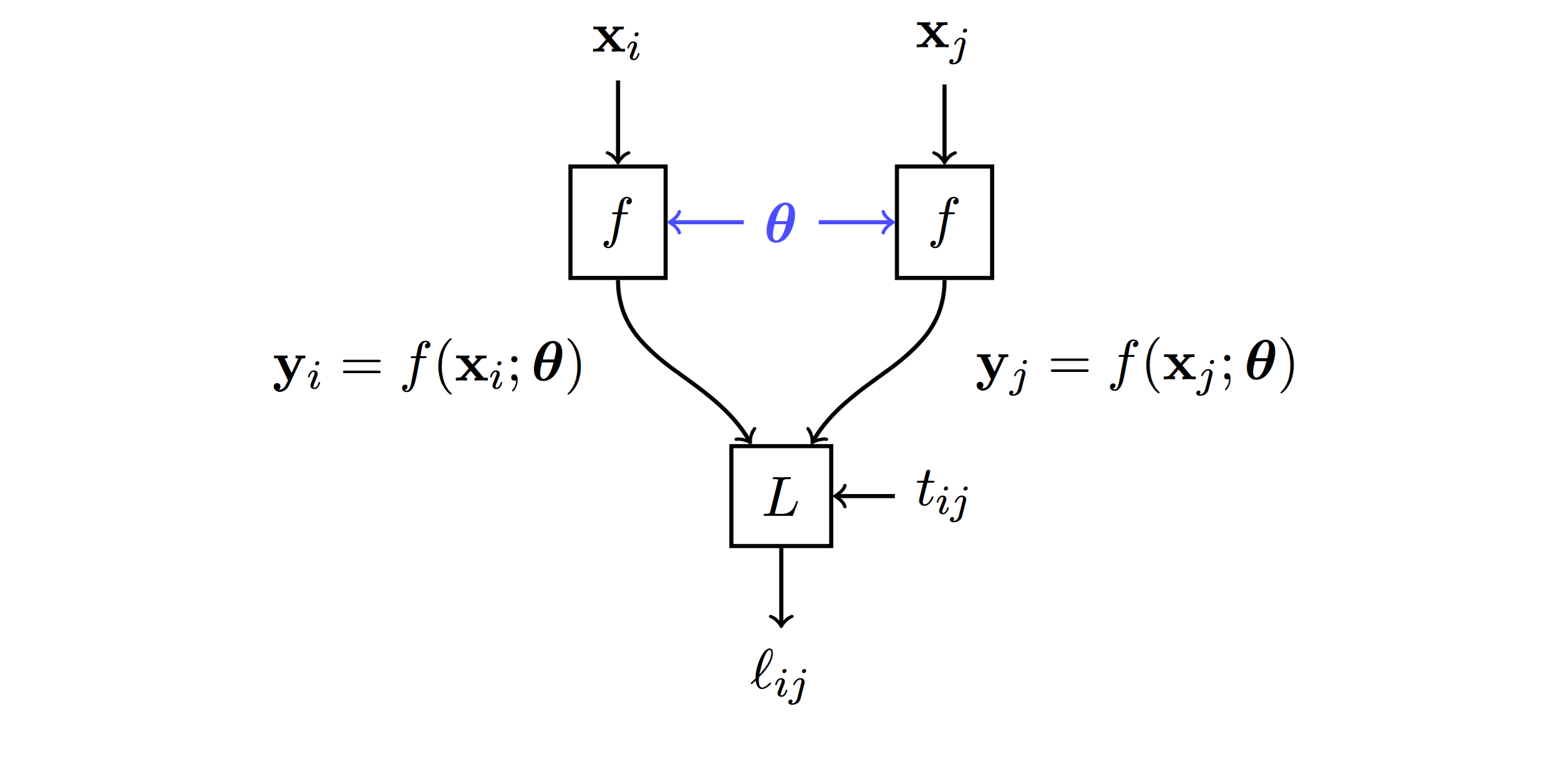] - an input sample is a _pair_ $( \mathbf{x}\_i, \mathbf{x}\_j)$ - both $\mathbf{x}\_i$, $\mathbf{x}\_j$ go through the _same_ function $f$ with _shared_ parameters $\theta$ - loss $\ell\_{ij}$ is measured on output pair $( \mathbf{y}\_i, \mathbf{y}\_j)$ and target $t\_{ij}$ .citation[ S. Chopra et al.,Learning a similarity metric discriminatively, with application to face verification, CVPR 2005] --- # Contrastive loss .center.width-60[] - input samples $\mathbf{x}\_i$, output vectors $\mathbf{y}\_i= f(\mathbf{x}\_i; \theta)$, target variables $t\_{ij}=\mathbb{1}[\text{sim}(\mathbf{x}\_i, \mathbf{x}\_j)]$ - _contrastive loss_ is a function of distance $\Vert \mathbf{y}\_i - \mathbf{y}\_j \Vert$ only $$\ell\_{ij} = L((\mathbf{y}\_i,\mathbf{y}\_j), t\_{ij} ) = \ell (\Vert \mathbf{y}\_i - \mathbf{y}\_j \Vert, t\_{ij})$$ .citation[ R. Hadsell et al., Dimensionality reduction by learning an invariant mapping, CVPR 2006] --- # Contrastive loss .center.width-60[] - input samples $\mathbf{x}\_i$, output vectors $\mathbf{y}\_i= f(\mathbf{x}\_i; \theta)$, target variables $t\_{ij}=\mathbb{1}[\text{sim}(\mathbf{x}\_i, \mathbf{x}\_j)]$ - _contrastive loss_ is a function of distance $\Vert \mathbf{y}\_i - \mathbf{y}\_j \Vert$ only $$\ell\_{ij} = L((\mathbf{y}\_i,\mathbf{y}\_j), t\_{ij} ) = \ell (\Vert \mathbf{y}\_i - \mathbf{y}\_j \Vert, t\_{ij})$$ - _similar_ samples are _attracted_ $$\ell(x,t)=\textcolor{red}{t\ell^{+}} + (1-t)\ell^{-}(x) = \textcolor{red}{t x^2} + (1-t)[m-x]^2\_+$$ .citation[ R. Hadsell et al., Dimensionality reduction by learning an invariant mapping, CVPR 2006] --- # Contrastive loss .center.width-60[] - input samples $\mathbf{x}\_i$, output vectors $\mathbf{y}\_i= f(\mathbf{x}\_i; \theta)$, target variables $t\_{ij}=\mathbb{1}[\text{sim}(\mathbf{x}\_i, \mathbf{x}\_j)]$ - _contrastive loss_ is a function of distance $\Vert \mathbf{y}\_i - \mathbf{y}\_j \Vert$ only $$\ell\_{ij} = L((\mathbf{y}\_i,\mathbf{y}\_j), t\_{ij} ) = \ell (\Vert \mathbf{y}\_i - \mathbf{y}\_j \Vert, t\_{ij})$$ - _dissimilar_ samples are _repelled_ if closer than margin $m$ $$\ell(x,t)=t\ell^{+} + (1-t)\textcolor{red}{\ell^{-}(x)} = t x^2 + (1-t)\textcolor{red}{[m-x]^2\_+}$$ .citation[ R. Hadsell et al., Dimensionality reduction by learning an invariant mapping, CVPR 2006] --- # Training siamese networks ## Data collection and loading - sample positive pairs $( \mathbf{x}\_i, \mathbf{x}\_j)$, with samples coming from the same class - sample negative pairs $( \mathbf{x}\_i, \mathbf{x}\_j)$, with samples of different classes - combine pairs of samples in larger mini-batches - __it's highly important to properly tune mini-batches__: balance positives and negatives, discard easy negatives and positives and focus on more difficult ones. .hidden[ ## Learning - pass all images through the two networks with shared parameters (in fact the same network) - backpropagate through the two networks and sum gradients from the two samples ] --- count: false # Training siamese networks ## Data collection and loading - sample positive pairs $( \mathbf{x}\_i, \mathbf{x}\_j)$, with samples coming from the same class - sample negative pairs $( \mathbf{x}\_i, \mathbf{x}\_j)$, with samples of different classes - combine pairs of samples in larger mini-batches - __it's highly important to properly tune mini-batches__: balance positives and negatives, discard easy negatives and positives and focus on more difficult ones. ## Learning - pass all images through the two networks with shared parameters (in fact the same network) - backpropagate through the two networks and sum gradients from the two samples --- # Triplet architecture .grid[ .kol-6-12[ .center.width-100[] ] .kol-6-12[ - an input sample is a _triple_ $(\mathbf{x}\_i, \mathbf{x}\_i^+, \mathbf{x}\_i^-)$ ] ] .citation[ Wang et al., Learning fine-grained image similarity with deep ranking, CVPR 2014] --- # Triplet architecture .grid[ .kol-6-12[ .center.width-100[] ] .kol-6-12[ - an input sample is a _triple_ $(\mathbf{x}\_i, \mathbf{x}\_i^+, \mathbf{x}\_i^-)$ - $\mathbf{x}\_i, \mathbf{x}\_i^+, \mathbf{x}\_i^-$ go through the _same_ function $f$ with _shared_ parameters $\theta$ ] ] .citation[ Wang et al., Learning fine-grained image similarity with deep ranking, CVPR 2014] --- # Triplet architecture .grid[ .kol-6-12[ .center.width-100[] ] .kol-6-12[ - an input sample is a _triple_ $(\mathbf{x}\_i, \mathbf{x}\_i^+, \mathbf{x}\_i^-)$ - $\mathbf{x}\_i, \mathbf{x}\_i^+, \mathbf{x}\_i^-$ go through the _same_ function $f$ with _shared_ parameters $\theta$ - loss $\ell\_i$ is measured on output triple $(\mathbf{y}\_i, \mathbf{y}\_i^+, \mathbf{y}\_i^-)$ ] ] .citation[ Wang et al., Learning fine-grained image similarity with deep ranking, CVPR 2014] --- # Triplet loss - input _anchor_ $\mathbf{x}\_i$, output $\mathbf{y}\_i = f(\mathbf{x}\_i; \theta)$; positive $\mathbf{y}\_i^+ = f(\mathbf{x}\_i^+; \theta)$, negative $\mathbf{y}\_i^- = f(\mathbf{x}\_i^-; \theta)$ - _triplet loss_ is a function of distances $\Vert \mathbf{y}\_i - \mathbf{y}\_i^+ \Vert$, $\Vert \mathbf{y}\_i - \mathbf{y}\_i^- \Vert$ only $$\ell\_i = L(\mathbf{y}\_i, \mathbf{y}\_i^+, \mathbf{y}\_i^-) =\ell(\Vert \mathbf{y}\_i - \mathbf{y}\_i^+ \Vert, \Vert \mathbf{y}\_i - \mathbf{y}\_i^- \Vert)$$ $$\ell(x^+, x^-) = [m + (x^+)^2 - (x^-)^2]\_+$$ so distance $\Vert \mathbf{y}\_i - \mathbf{y}\_i^+ \Vert$ should be less than $\Vert \mathbf{y}\_i - \mathbf{y}\_i^- \Vert$ by _margin_ $m$ .citation[ Wang et al., Learning fine-grained image similarity with deep ranking, CVPR 2014] --- # Triplet loss - input _anchor_ $\mathbf{x}\_i$, output $\mathbf{y}\_i = f(\mathbf{x}\_i; \theta)$; positive $\mathbf{y}\_i^+ = f(\mathbf{x}\_i^+; \theta)$, negative $\mathbf{y}\_i^- = f(\mathbf{x}\_i^-; \theta)$ - _triplet loss_ is a function of distances $\Vert \mathbf{y}\_i - \mathbf{y}\_i^+ \Vert$, $\Vert \mathbf{y}\_i - \mathbf{y}\_i^- \Vert$ only $$\ell\_i = L(\mathbf{y}\_i, \mathbf{y}\_i^+, \mathbf{y}\_i^-) =\ell(\Vert \mathbf{y}\_i - \mathbf{y}\_i^+ \Vert, \Vert \mathbf{y}\_i - \mathbf{y}\_i^- \Vert)$$ $$\ell(x^+, x^-) = [m + (x^+)^2 - (x^-)^2]\_+$$ so distance $\Vert \mathbf{y}\_i - \mathbf{y}\_i^+ \Vert$ should be less than $\Vert \mathbf{y}\_i - \mathbf{y}\_i^- \Vert$ by _margin_ $m$ - by taking _two pairs_ $(\mathbf{x}\_i, \mathbf{x}\_i^+)$ and $(\mathbf{x}\_i, \mathbf{x}\_i^-)$ at a time with targets $1$, $0$ respectively, the _contrastive loss_ can be writen similarly $$\ell(x^+, x^-) = (x^+)^2 + [m-x^-]^2\_+$$ so distance $\Vert \mathbf{y}\_i - \mathbf{y}\_i^+ \Vert$ should be small and $\Vert \mathbf{y}\_i - \mathbf{y}\_i^- \Vert$ larger than $m$ .citation[ Wang et al., Learning fine-grained image similarity with deep ranking, CVPR 2014] --- count: false # Training with the triplet loss $$\ell\_i = L(\mathbf{y}\_i, \mathbf{y}\_i^+, \mathbf{y}\_i^-) =\ell(\Vert \mathbf{y}\_i - \mathbf{y}\_i^+ \Vert, \Vert \mathbf{y}\_i - \mathbf{y}\_i^- \Vert)$$ - sample a mini-batch of triplets$(\mathbf{x}\_i, \mathbf{x}\_i^+, \mathbf{x}\_i^-)$ - forward pass on all $3$ networks - compute loss over all samples and sum gradients for updating weights --- # Siamese networks .grid[ .kol-6-12[ ``` class SiameseNet(nn.Module): def __init__(self, embedding_net): super(SiameseNet, self).__init__() self.embedding_net = embedding_net def forward(self, x1, x2): output1 = self.embedding_net(x1) output2 = self.embedding_net(x2) return output1, output2 def get_embedding(self, x): return self.embedding_net(x) ``` ] .kol-6-12[ ``` class TripletNet(nn.Module): def __init__(self, embedding_net): super(TripletNet, self).__init__() self.embedding_net = embedding_net def forward(self, x1, x2, x3): output1 = self.embedding_net(x1) output2 = self.embedding_net(x2) output3 = self.embedding_net(x3) return output1, output2, output3 def get_embedding(self, x): return self.embedding_net(x) ``` ] ] --- count:false # Siamese networks .grid[ .kol-6-12[ ``` class SiameseNet(nn.Module): def __init__(self, embedding_net): super(SiameseNet, self).__init__() self.embedding_net = embedding_net def forward(self, x1, x2): * output1 = self.embedding_net(x1) * output2 = self.embedding_net(x2) return output1, output2 def get_embedding(self, x): return self.embedding_net(x) ``` ] .kol-6-12[ ``` class TripletNet(nn.Module): def __init__(self, embedding_net): super(TripletNet, self).__init__() self.embedding_net = embedding_net def forward(self, x1, x2, x3): * output1 = self.embedding_net(x1) * output2 = self.embedding_net(x2) * output3 = self.embedding_net(x3) return output1, output2, output3 def get_embedding(self, x): return self.embedding_net(x) ``` ] ] --- # Hard negative sampling After a few epochs, If $(\mathbf{x}\_i, \mathbf{x}\_i^{+}, \mathbf{x}\_i^{-})$ are chosen randomly, it will be easy to satisfy the inequality in the loss. -- Gradients in one batch quickly become almost $0$ except for **hard cases**. Random sampling is inefficient to find these hard cases -- count: false - **Hard triplet sampling:** sample $\mathbf{x}\_i^{-}$ such that: $$||\mathbf{y} - \mathbf{y}^{+}|| > ||\mathbf{y} - \mathbf{y}^{-}|| + m$$ - **Semi Hard triplet sampling:** sample $\mathbf{x}\_i^{-}$ such that: $$||\mathbf{y} - \mathbf{y}^{+}|| > ||\mathbf{y} - \mathbf{y}^{-}||$$ --- class: middle, center # Applications --- # Face recognition .center.width-25[] - A threshold is computed on test set to decide which faces are the same - Best model achieves 99.6% verification accuracy on Labeled Faces in the Wild dataset - Works well even with non-camera facing faces .citation[F. Schroff et al., Facenet: A unified embedding for face recognition and clustering, CVPR 2015 ] --- # Deep image retrieval .center.width-70[] .citation[A. Gordo et al., Deep Image Retrieval: Learning Global Representations for Image Search, ECCV 2016 ] - query $\mathbf{x}\_i$, relevant $\mathbf{x}\_i^+$ (same building), irrelevant $\mathbf{x}\_i^-$ (other building) --- count: false # Deep image retrieval .center.width-70[] .citation[A. Gordo et al., Deep Image Retrieval: Learning Global Representations for Image Search, ECCV 2016 ] - query $\mathbf{x}\_i$, relevant $\mathbf{x}\_i^+$ (same building), irrelevant $\mathbf{x}\_i^-$ (other building) --- count: false # Deep image retrieval .center.width-70[] .citation[A. Gordo et al., Deep Image Retrieval: Learning Global Representations for Image Search, ECCV 2016 ] - query $\mathbf{x}\_i$, relevant $\mathbf{x}\_i^+$ (same building), irrelevant $\mathbf{x}\_i^-$ (other building) - triplet loss is evaluated on output $(\mathbf{y}\_i, \mathbf{y}\_i^+, \mathbf{y}\_i^-)$ --- # Patch matching .center.width-45[] --- # Patch matching .center.width-70[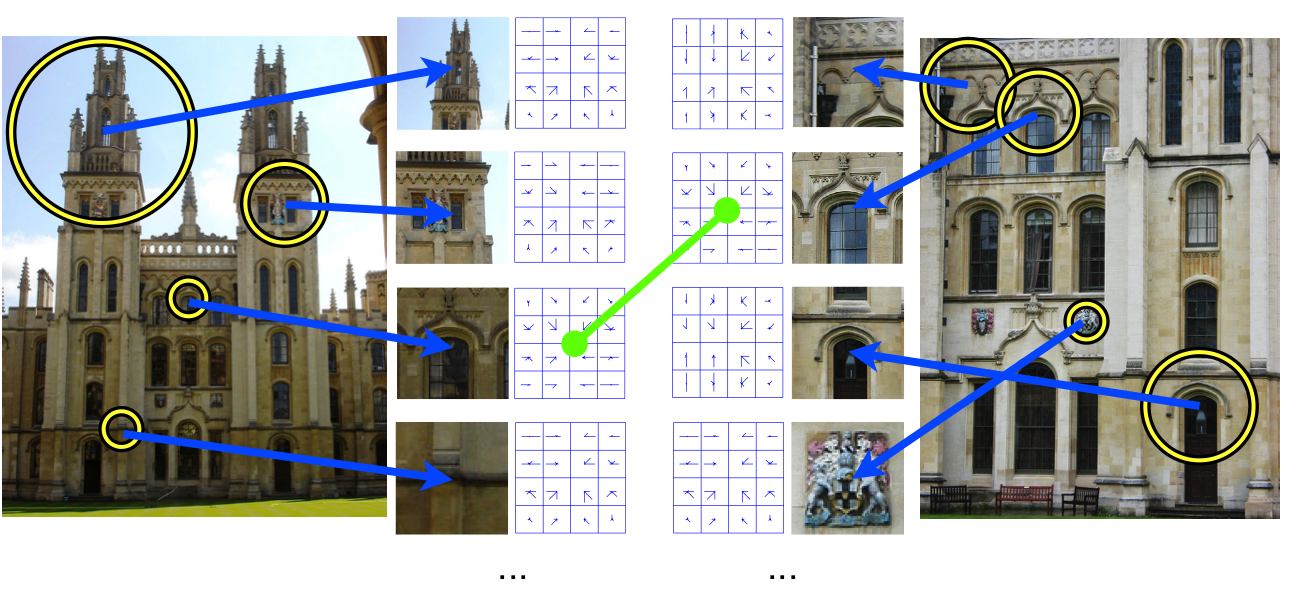] .credit[Figure credit: A. Vedaldi] --- # Patch matching .center.width-60[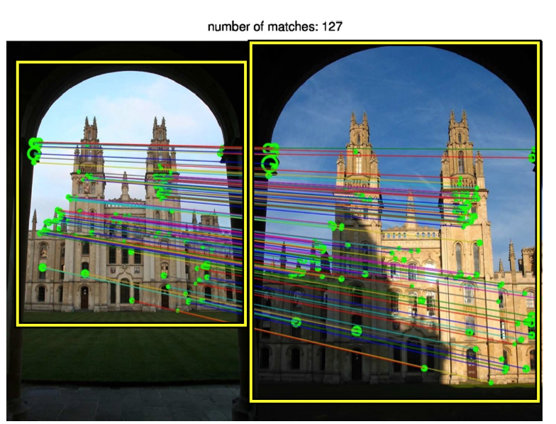] .credit[Figure credit: A. Vedaldi] --- # Image reconstruction .center.width-70[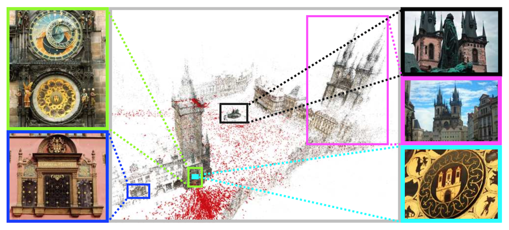] .caption[Structure from motion] .citation[F. Radenovic et al., CNN Image Retrieval Learns From BoW: Unsupervised Fine-Tuning with Hard Examples, ECCV 2016 <br/> Schonberger et al., From Single Image Query to Detailed 3D Reconstruction, CVPR 2015.] --- # Person re-identification .grid[ .kol-6-12[ .center.width-70[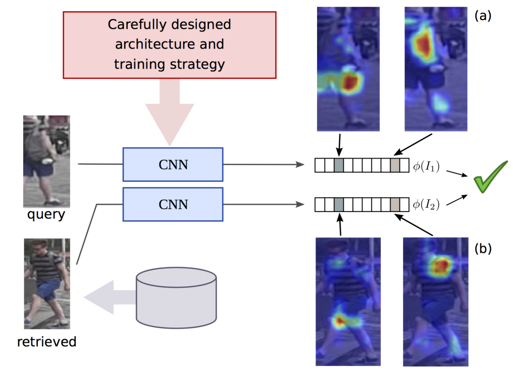] ] .kol-6-12[ ] ] .citation[J. Almazan et al., Re-ID Done Right: towards Good Practices for Person re-Identification, arXiv 2018] --- count: false # Person re-identification .grid[ .kol-6-12[ .center.width-70[] ] .kol-6-12[ .center.width-70[] ] ] .citation[J. Almazan et al., Re-ID Done Right: towards Good Practices for Person re-Identification, arXiv 2018] --- class: middle, center .big[Going beyond pairs and triplets ...] --- # N-pair loss .center.width-70[] .caption[Deep metric learning with (left) triplet loss and (right) $(N+1)$-tuplet loss. <br/>$(N+1)$-tuplet loss pushes $N-1$ negative examples all at once.] - generalize *triplet-loss* with **N-pair loss** - sample pairs of similar examples and use as negative all the other samples in the mini-batch .citation[K. Sohn, Improved Deep Metric Learning with Multi-class N-pair Loss Objective, NeurIPS 2016] --- ## Exemplar networks .center.bigger.blue[The image on the left is a distorted crop extracted from an image, which of these crops has the same source image?] .hidden.center.bigger.red[Easy if robust to the desired transformations (geometry and colour) ] .grid[ .kol-4-12[ <br/> .center.width-25[] ] .kol-8-12[ .center.width-100[] ] ] .citation[A. Dosovitskiy et al., Discriminative Unsupervised Feature Learning with Exemplar Convolutional Neural Networks, PAMI 2015] --- count: false ## Exemplar networks .center.bigger.blue[The image on the left is a distorted crop extracted from an image, which of these crops has the same source image?] .center.bigger.red[Easy if robust to the desired transformations (geometry and colour) ] .grid[ .kol-4-12[ <br/> .center.width-25[] ] .kol-8-12[ .center.width-100[] ] ] .citation[A. Dosovitskiy et al., Discriminative Unsupervised Feature Learning with Exemplar Convolutional Neural Networks, PAMI 2015] --- ## Exemplar networks .grid[ .kol-4-12[ .center.width-70[] ] .kol-8-12[ .bigger.green[Pros] - Representations are invariant to desired transformations - Requires preservation of fine-grained information .bigger.red[Cons] - Choosing the augmentations is important - Exemplar based: images of the same class or instance are negatives - Nothing prevents it from focusing on the background - Original formulation is not scalable (number of “classes” = dataset size) ] ] .citation[A. Dosovitskiy et al., Discriminative Unsupervised Feature Learning with Exemplar Convolutional Neural Networks, PAMI 2015] --- class: middle ## Some notations Let $\mathbf{x} \in \mathcal{X}$ be input data and $y \in \\{1, \dots, L\\}$ and $f\_{\theta}(\cdot):\mathcal{X}\rightarrow\mathbb{R}^D$ a network generating an embedding vector $f\_{\theta}(\mathbf{x})$. <!-- We use $x^{+}$ and $\\{x^{i}\\}$ to denote a positive sample and set of negative examples for $x$. --> We denote: - $q=f\_{\theta}(\mathbf{x})$ (*query*) - $\\{\mathbf{x}^{i}\\}$ a set of samples from $\mathcal{X}$. - $k\_{i} = f\_{\theta}(\mathbf{x}^{i})$ the embeddings of $\\{\mathbf{x}^{i}\\}$ as keys (*representations*) --- ## Exemplar networks .grid[ .kol-3-12[ .center.width-90[] ] .kol-9-12[ Exemplar ConvNets are not scalable (number of “classes” = number of training images) - Using $w\_i$ as class prototype prevents explicit comparison between instances, i.e. individual samples - We can use instead a _non-parametric_ variant that replaces $q^\top w\_j$ with $q^\top k\_i$ $$\mathcal{L}\_{\text{softmax}} (q, c(q)) = - \log\frac{\exp(q^\top w\_{c(q)})}{ \sum\_{c\in C}\exp(q^\top w\_{c})}$$ $$\downarrow$$ $$\mathcal{L}\_{\text{non-param-softmax}}(q) = - \log \frac{\exp(q^\top k\_q )}{ \sum\_{i \in N}\exp(q ^\top k\_{i})}$$ ] ] .citation[A. Dosovitskiy et al., Discriminative Unsupervised Feature Learning with Exemplar Convolutional Neural Networks, PAMI 2015] --- count: false ## Exemplar networks .grid[ .kol-3-12[ .center.width-90[] ] .kol-9-12[ - $N$ is the number of training samples; $C$ is the number of classes - $c(q)$ is the class index of $q$ - $k\_q \in \\{ k\_i\\}$ is the key of a positive sample for $q$ $$\mathcal{L}\_{\text{softmax}} (q, c(q)) = - \log\frac{\exp(q^\top w\_{c(q)})}{ \sum\_{c\in C}\exp(q^\top w\_{c})}$$ $$\downarrow$$ $$\mathcal{L}\_{\text{non-param-softmax}}(q) = - \log \frac{\exp(q^\top k\_q )}{ \sum\_{i \in N}\exp(q ^\top k\_{i})}$$ ] ] .citation[A. Dosovitskiy et al., Discriminative Unsupervised Feature Learning with Exemplar Convolutional Neural Networks, PAMI 2015] --- # Histogram loss .center.width-70[] - for a mini-batch compute all pairwise positive similarities and negative similarities - compile similarities into distributions (differentiable approximations of distributions) - the loss aims to repell the two distributions .citation[E. Ustinova et al., Learning Deep Embeddings with Histogram Loss, NeurIPS 2016] --- class: middle, center ## Few classes, few labels --- # Prototypical networks Learns to extract class prototype vectors: - class prototype vector = mean feature vector of training examples - classify test example to the class with the closest prototype ($L\_2$ distance) - prototype vectors are similar to classification weights of networks .grid[ .kol-8-12[ Prototype vector of $k$-th class: $c\_k=\frac{1}{|S\_k|} \sum\_{(\mathbf{x}\_i, y\_i) \in S\_k} f\_{\theta}(\mathbf{x}\_i)$ Classification for example $x$: $$p\_{\theta}(y=k|\mathbf{x}) = \frac{\exp(-d(f\_{\theta}(\mathbf{x}), c\_k))}{\sum\_{k'}\exp(-d(f\_{\theta}(\mathbf{x}), c\_{k'}))}$$ ] .kol-4-12[ .center.width-70[] ] ] .citation[J Snell et al., Prototypical Networks for Few-shot Learning, NeurIPS 2017] --- class: middle, center ## Some classes with labels and some without labels --- # Imprinting .grid[ .kol-6-12[ .center.width-90[] ] .kol-6-12[ The cosine classifier $$p\_{\theta}(y=k|\mathbf{x}) = \frac{\exp(\tau f\_{\theta}(\mathbf{x})^\top w\_k )} { \sum\_{k'}\exp(\tau f\_{\theta}(\mathbf{x})^\top w\_{k'} )}$$ All vectors and weights are $L\_2$-normalized before the last layer ] ] .citation[H. Qi et al., Low-Shot Learning with Imprinted Weights, CVPR 2018 <br> S. Gidaris et al., Dynamic Few-Shot Visual Learning without Forgetting, CVPR 2018] --- count: false # Imprinting .grid[ .kol-6-12[ .center.width-90[] ] .kol-6-12[ .center.width-100[] .caption[ _left_: before imprinting; _right_: after imprinting] ] ] .citation[H. Qi et al., Low-Shot Learning with Imprinted Weights, CVPR 2018 <br> S. Gidaris et al., Dynamic Few-Shot Visual Learning without Forgetting, CVPR 2018] --- count: false # Imprinting .grid[ .kol-6-12[.center.width-90[] ] .kol-6-12[ - use network as feature extractor, train as usual - for new class, compute average embedding vector - use embedded vector as new class proxy/template - can be also fine-tuned later on ] ] .citation[H. Qi et al., Low-Shot Learning with Imprinted Weights, CVPR 2018 <br> S. Gidaris et al., Dynamic Few-Shot Visual Learning without Forgetting, CVPR 2018] --- # Imprinting ## Results .grid[ .kol-6-12[ .center[<img src="images/part13/imprinting_results3.png" style="width: 370px;" />] ] .kol-6-12[ .center[<img src="images/part13/imprinting_results4.png" style="width: 370px;" />] ] ] .citation[H. Qi et al., Low-Shot Learning with Imprinted Weights, CVPR 2018 <br> S. Gidaris et al., Dynamic Few-Shot Visual Learning without Forgetting, CVPR 2018] --- # Take-aways - .big[A specific type of architectures suitable for representation learning] - .big[In case of many classes and class imbalance, siamese networks might be better, while for standard settings use classification] - .big[Modern methods leverage siamese networks for unsupervised learning, where the network must recognize a perturbed sample in a large pool of negatives.] --- class: middle, center # Multi-modal siamese networks --- # CLIP .center.width-50[] .center[Training an image network and a text network together from $400M$ pairs of images and captions crawled from Internet] .citation[A. Radford et al., Learning Transferable Visual Models From Natural Language Supervision, arXiv 2021 ] --- # CLIP .center.width-55[] .center[Use networks and embeddings in *zero-shot* classification] .citation[A. Radford et al., Learning Transferable Visual Models From Natural Language Supervision, arXiv 2021 ] --- class: middle ## Implementation - numpy-like pseudocode ```python # image_encoder - ResNet or Vision Transformer # text_encoder - CBOW or Text Transformer # I[n, h, w, c] - minibatch of aligned images # T[n, l] - minibatch of aligned texts # W_i[d_i, d_e] - learned proj of image to embed # W_t[d_t, d_e] - learned proj of text to embed # t - learned temperature parameter # extract feature representations of each modality I_f = image_encoder(I) #[n, d_i] T_f = text_encoder(T) #[n, d_t] # joint multimodal embedding [n, d_e] I_e = l2_normalize(np.dot(I_f, W_i), axis=1) T_e = l2_normalize(np.dot(T_f, W_t), axis=1) # scaled pairwise cosine similarities [n, n] logits = np.dot(I_e, T_e.T) * np.exp(t) # symmetric loss function labels = np.arange(n) loss_i = cross_entropy_loss(logits, labels, axis=0) loss_t = cross_entropy_loss(logits, labels, axis=1) loss = (loss_i + loss_t)/2 ``` .citation[A. Radford et al., Learning Transferable Visual Models From Natural Language Supervision, arXiv 2021 ] --- class: middle ## Works very well in practice .center.width-40[] .caption[Zero-shot CLIP is competitive with a fully supervised baseline] .citation[A. Radford et al., Learning Transferable Visual Models From Natural Language Supervision, arXiv 2021 ] --- class: middle Training CLIP is very expensive: - ResNet (`RN50x64`): $18$ days on $592$ V100 GPUS - ViT (Vision Transformer): $12$ days on $256$ V100 GPUs - batch-size: $32.768$ Such models that are expensive to train but can be repurposed for other tasks, are referred to as *foundation models*. .citation[R. Bommasani et al., On the Opportunities and Risks of Foundation Models, arXiv 2021] --- # CLIPStyler .center.width-65[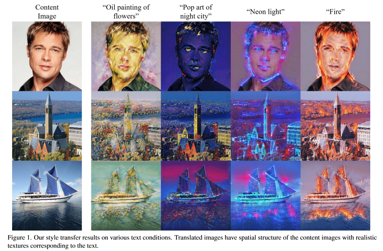] .center[Change style of image using text only] .citation[Kwon et al., CLIPstyler: Image Style Transfer with a Single Text Condition, CVPR 2022] --- # CLIPStyler .center.width-65[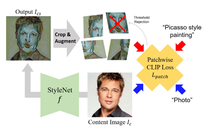] .center[Content is preserved thanks to alingnment in CLIP space] .citation[Kwon et al., CLIPstyler: Image Style Transfer with a Single Text Condition, CVPR 2022] --- # CLIPStyler .center.width-75[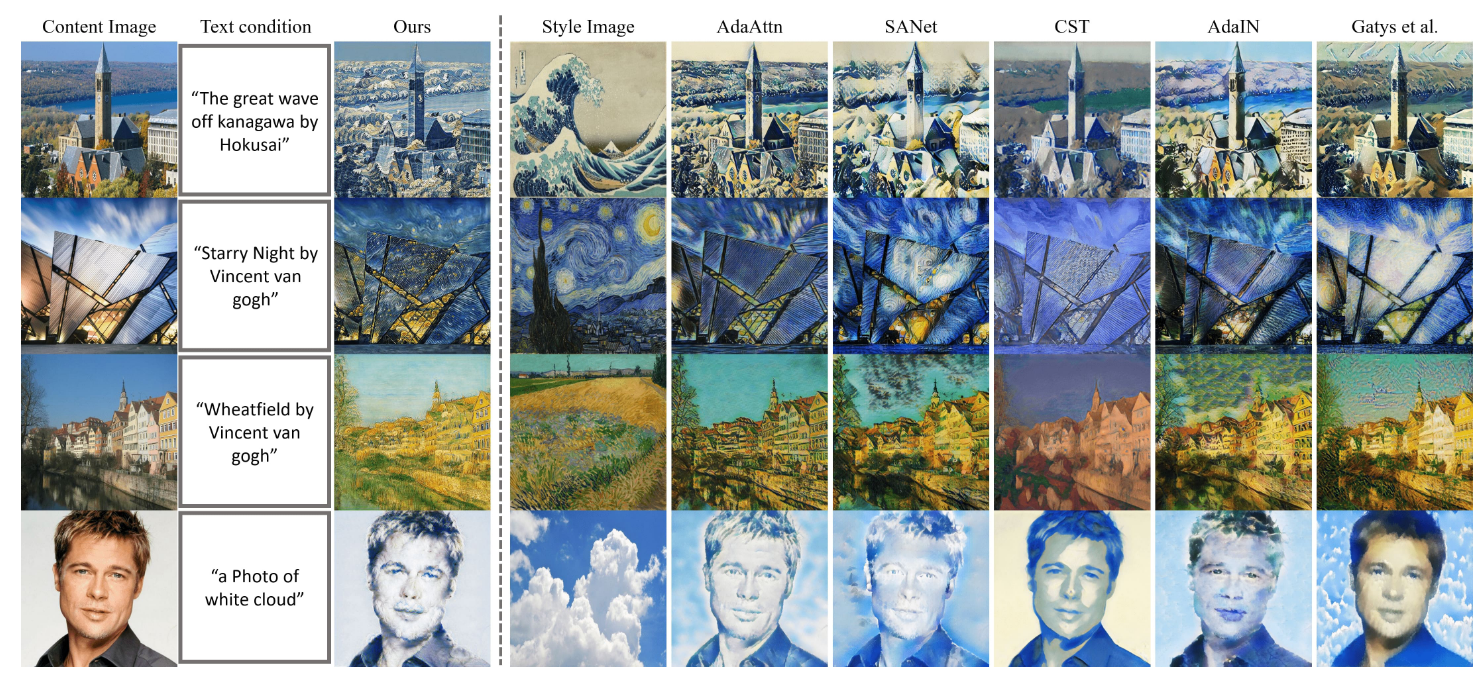] .center[Works similarly with image based styling] .citation[Kwon et al., CLIPstyler: Image Style Transfer with a Single Text Condition, CVPR 2022] --- # FlexIT .center.width-90[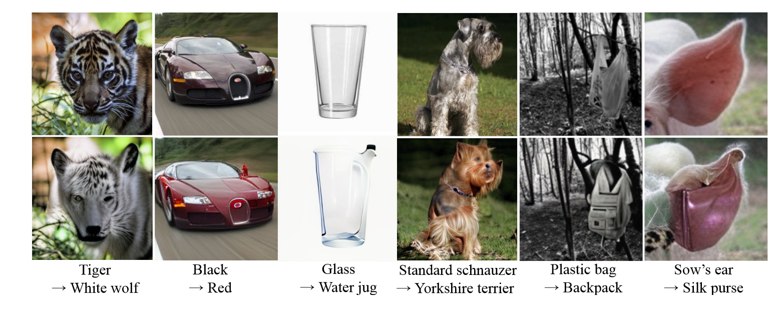] .center[Transform image using text indication] .citation[Couairon et al., FlexIT: Towards Flexible Semantic Image Translation, CVPR 2022] --- # FlexIT .center.width-90[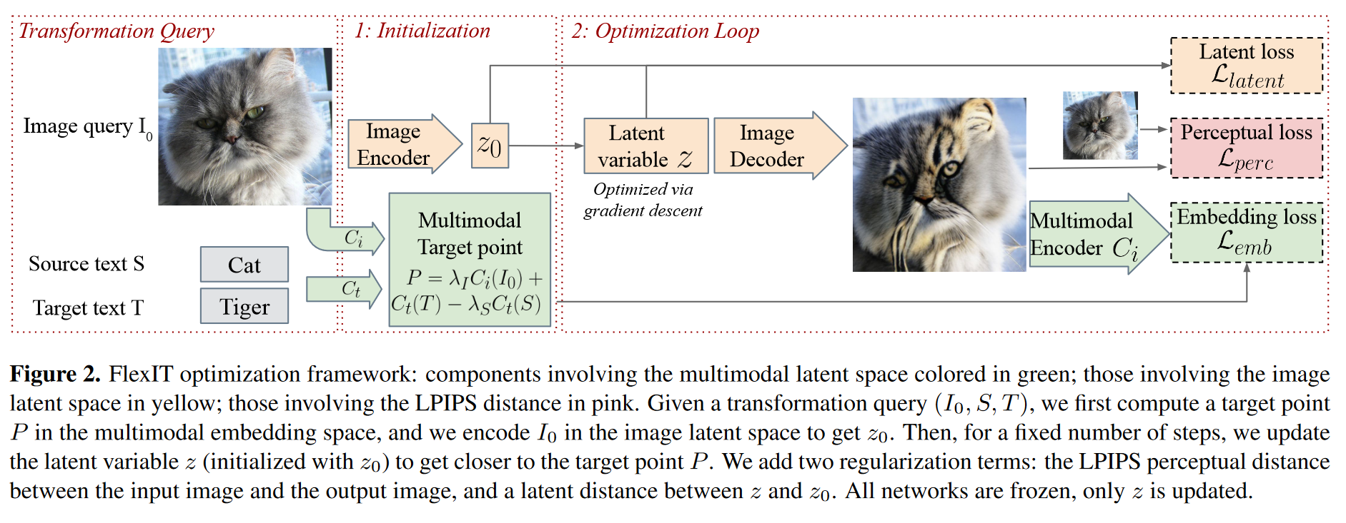] .center[Optimize latent variable only from a pre-trained generative model to steer it towards generativ what we want] .citation[Couairon et al., FlexIT: Towards Flexible Semantic Image Translation, CVPR 2022] --- # Prompt-driven Zero-shot Domain Adaptation .center.width-90[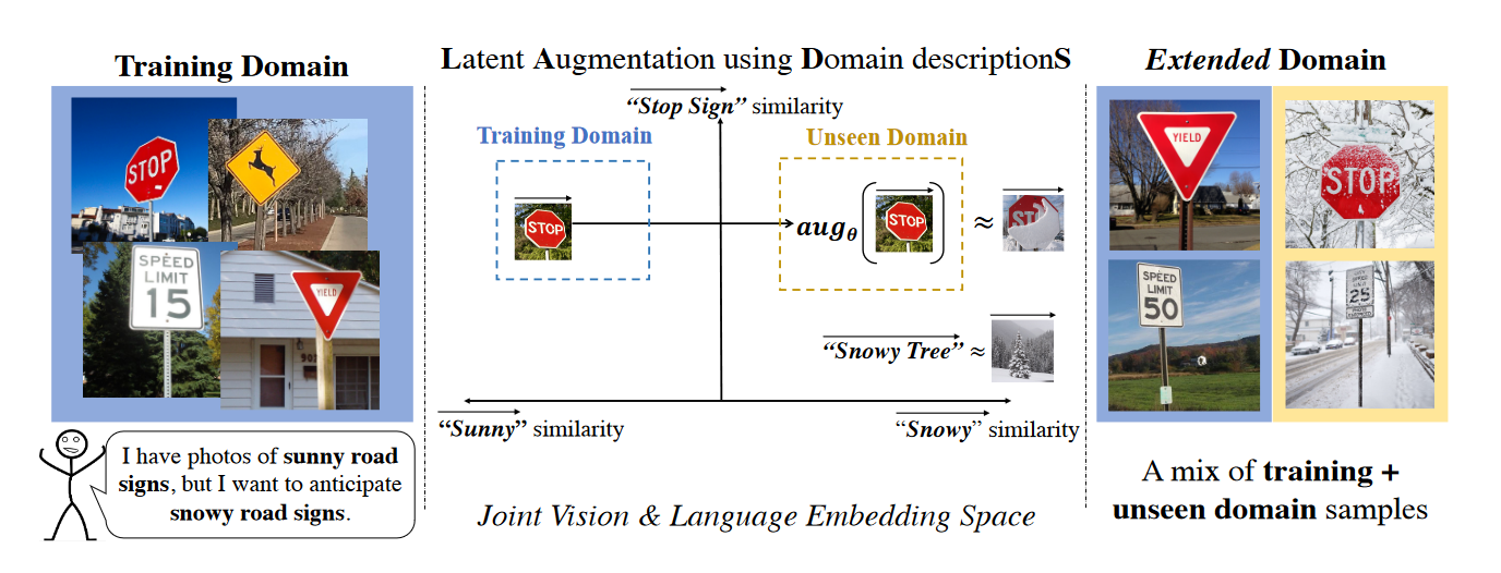] .center[Use textual information to generate features for domains we have seen yet] .citation[Dunlap et al., Using Language to Extend to Unseen Domainsn, ICLR 2023 <br> Fahes et al., PØDA: Prompt-driven Zero-shot Domain Adaptation, arXiv 2022] --- # Prompt-driven Zero-shot Domain Adaptation .center.width-90[] .center[Use textual information to generate features for domains we have seen yet] .citation[Dunlap et al., Using Language to Extend to Unseen Domainsn, ICLR 2023 <br> Fahes et al., PØDA: Prompt-driven Zero-shot Domain Adaptation, arXiv 2022] --- # Prompt-driven Zero-shot Domain Adaptation .center.width-100[] .center[Use textual information to generate features for domains we have seen yet] .citation[Dunlap et al., Using Language to Extend to Unseen Domainsn, ICLR 2023 <br> Fahes et al., PØDA: Prompt-driven Zero-shot Domain Adaptation, arXiv 2022] --- # Stable Diffusion .center.width-80[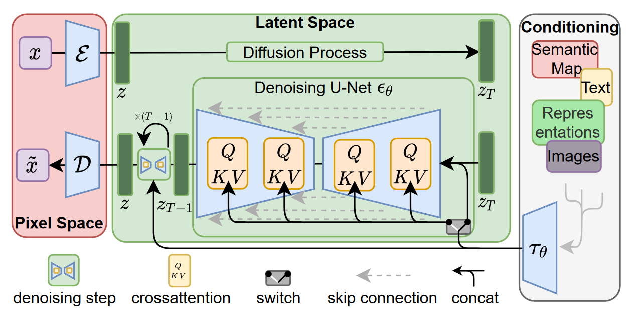] .center[Condition image generation on text embeddings from CLIP] .citation[Rombach et al., High-Resolution Image Synthesis With Latent Diffusion Models, CVPR 2022] --- # Stable Diffusion .center.width-100[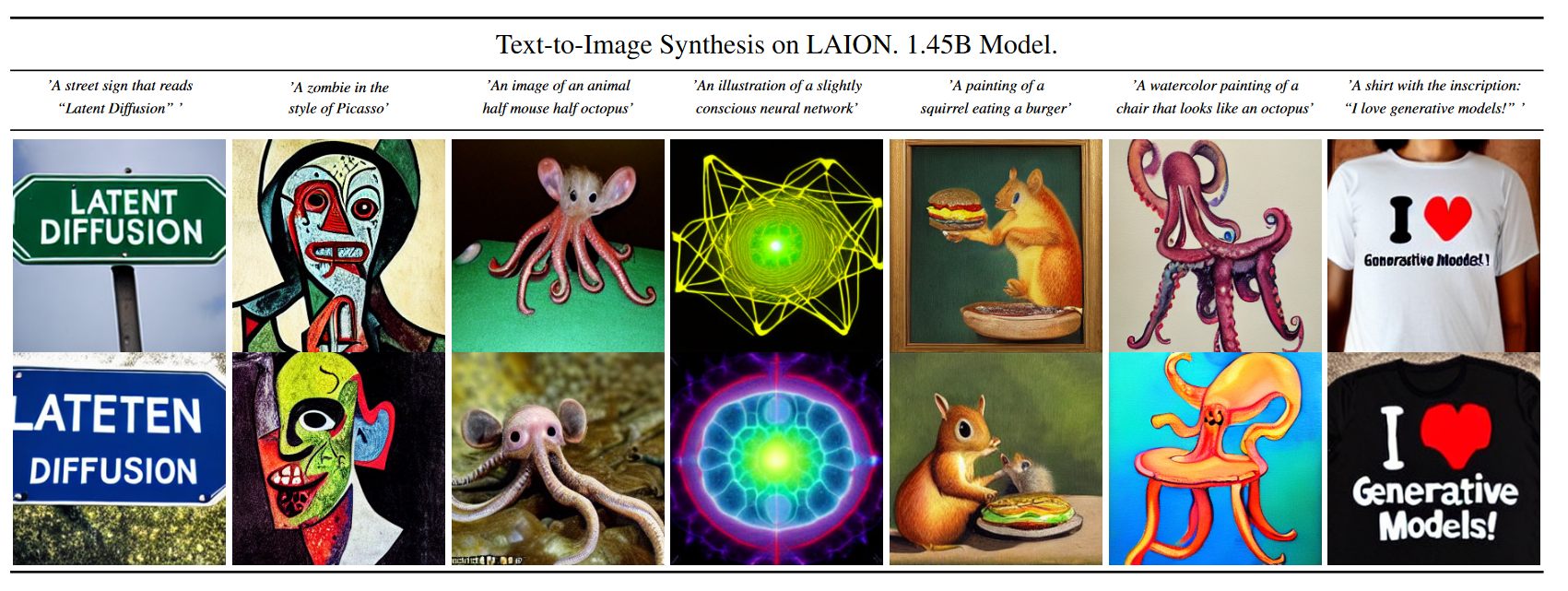] .center[Text to image synthesis examples -- starting to very dated] .citation[Rombach et al., High-Resolution Image Synthesis With Latent Diffusion Models, CVPR 2022] --- class: middle, center .bigger[CLIP is currently widely used in various computer vision and text tasks to kickstart or steer learning.] .bigger[Intuitively the structured learned in the feature space from language can effectively steer visual representation more than simple individual labels.] --- class: end-slide, center count: false The end.