layout: true .center.footer[Andrei BURSUC and Relja ARANDJELOVIĆ | Self-Supervised Learning] --- class: center, middle, title-slide count: false ## .bold[CVPR 2020 Tutorial] # Towards Annotation-Efficient Learning # Self-Supervised Learning <br> .grid[ .kol-2-12[ ] .kol-4-12[ .center.big.bold[Andrei Bursuc] <br> <br> <!-- .width-5[] --> .center[<img src="images/logo_valeoai.png" style="width: 200px;" />] ] .kol-4-12[ .center.big.bold[Relja Arandjelović] <br> <br> .center[<img src="images/logo_deepmind.png" style="width: 230px;" />] ] .kol-2-12[ ] ] .foot[https://annotation-efficient-learning.github.io/] <!-- <div class="footer-logo"><img src="images/logo_cvpr.png" style="width: 250px;"/></div> --> <div class="header-logo"><img src="images/logo_cvpr.png" style="width: 250px;"/></div> --- class: middle # Self-Supervised Learning ## 1. Motivation ## 2. A tour of pretext tasks for Self-Supervised Learning ## 3. Practical considerations ## 4. Evaluation ## 5. Applications --- class: middle, center # 1. Motivation <!-- .bigg.highlight[Andrei] --> --- count: false class: middle, center .center.big[Deep Learning + Supervised Learning is a really cool and strong combo.] .hidden.center.big.italic[... when task and data permit it.] --- count: false class: middle .center.big[Deep Learning + Supervised Learning is a really cool and strong combo.] .center.big[... when task and data permit it.] --- class: middle .center.big[In addition to **data acquisition and annotation challenges**, <br/>the _representation learning perspective_ provides additional reasons <br/> to look for alternative or complementary solutions. ] --- class: middle ## .center[The type of supervision signal can bias the network in unexpected ways] .center.width-90[] .caption[VGG-16 preditions on original and artificially texturised images.] .citation[L.A. Gatys et al., Texture and art with deep neural networks, Neurobiology 2017] --- class: middle ## .center[The type of supervision signal can bias the network in unexpected ways] .center.width-85[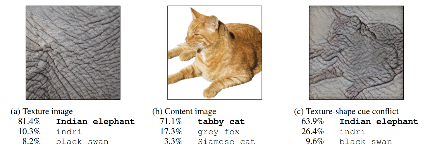] .caption[Classification predictions of a ResNet-50 trained on ImageNet] .citation[R. Geirhos et al., ImageNet-trained CNNs are biased towards texture; increasing shape bias improves accuracy and robustness, ICLR 2019] --- class: middle, center .big[Improving representation learning requires features that are *not specialized for solving a particular supervised task*, but rather *encapsulate richer statistics for various downstream tasks*.] --- class: middle ## .center[The success of self-supervised methods in NLP, e.g. _word2vec_, is inspiring ] .center.width-85[] .caption[Missing word prediction task.] .center.width-85[] .caption[Next sentence prediction task.] .citation[T. Mikolov et al., Efficient estimation of word representations in vector space, ArXiv 2013 <br/>T. Mikolov et al., Distributed representations of words and phrases and their compositionality, NeurIPS 2013<br/>J. Devlin, BERT: Pre-training of Deep Bidirectional Transformers for Language Understanding, ArXiv 2018] --- count: false class: middle # .center[What is self-supervision?] <br/> - .bigger[A form of unsupervised learning where the **data (not the human) provides the supervision signal**] .hidden[ - .bigger[Usually, *define a pretext task* for which the network is forced to learn what we really care about] ] .hidden[ - .bigger[For most pretext tasks, *a part of the data is withheld* and the network has to predict it] ] .hidden[ - .bigger[The features/representations learned on the pretext task are subsequently used for a different *downstream task*, usually where some annotations are available.] ] --- count: false class: middle # .center[What is self-supervision?] <br/> - .bigger[A form of unsupervised learning where the **data (not the human) provides the supervision signal**] - .bigger[Usually, *define a pretext task* for which the network is forced to learn what we really care about] .hidden[ - .bigger[For most pretext tasks, *a part of the data is withheld* and the network has to predict it] ] .hidden[ - .bigger[The features/representations learned on the pretext task are subsequently used for a different *downstream task*, usually where some annotations are available.] ] --- count: false class: middle # .center[What is self-supervision?] <br/> - .bigger[A form of unsupervised learning where the **data (not the human) provides the supervision signal**] - .bigger[Usually, *define a pretext task* for which the network is forced to learn what we really care about] - .bigger[For most pretext tasks, *a part of the data is withheld* and the network has to predict it] .hidden[ - .bigger[The features/representations learned on the pretext task are subsequently used for a different *downstream task*, usually where some annotations are available.] ] --- count: false class: middle # .center[What is self-supervision?] <br/> - .bigger[A form of unsupervised learning where the **data (not the human) provides the supervision signal**] - .bigger[Usually, *define a pretext task* for which the network is forced to learn what we really care about] - .bigger[For most pretext tasks, *a part of the data is withheld* and the network has to predict it] - .bigger[The features/representations learned on the pretext task are subsequently used for a different *downstream task*, usually where some annotations are available.] --- class: middle ## .center[Example: Rotation prediction] .center.width-70[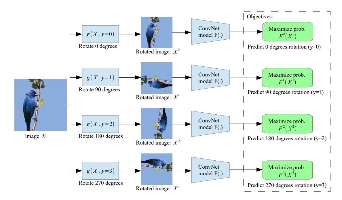] .center[Predict the orientation of the image] .citation[S. Gidaris et al., Unsupervised Representation Learning by Predicting Image Rotations, ICLR 2018] --- # Self-supervised learning pipeline .center.bold.bigger[*Stage 1:* Train network on pretext task (without human labels)] .center.width-90[] --- count:false # Self-supervised learning pipeline .center.bold.bigger[*Stage 1:* Train network on pretext task (without human labels) ] .center.width-90[] .center.bold.bigger[*Stage 2:* Train classifier on learned features for new task with fewer labels] .center.width-90[] --- count:false # Self-supervised learning pipeline .center.bold.bigger[*Stage 1:* Train network on pretext task (without human labels)] .center.width-90[] .center.bold.bigger[*Stage 2:* Fine-tune network for new task with fewer labels] .center.width-90[] --- class: middle, black-slide ## .center[Karate Kid and Self-Supervised Learning] .center.width-85[] .caption[The Karate Kid (1984)] --- class: middle, black-slide ## .center[Stage 1: Train .italic[muscle memory] on pretext tasks] .grid[ .kol-4-12[ .center.width-100[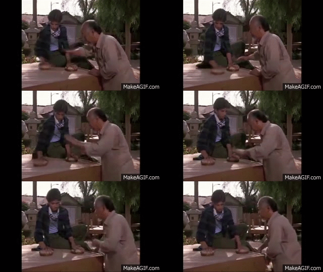] ] .kol-4-12[ .center.width-100[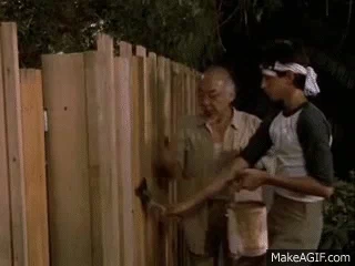] ] .kol-4-12[ .center.width-100[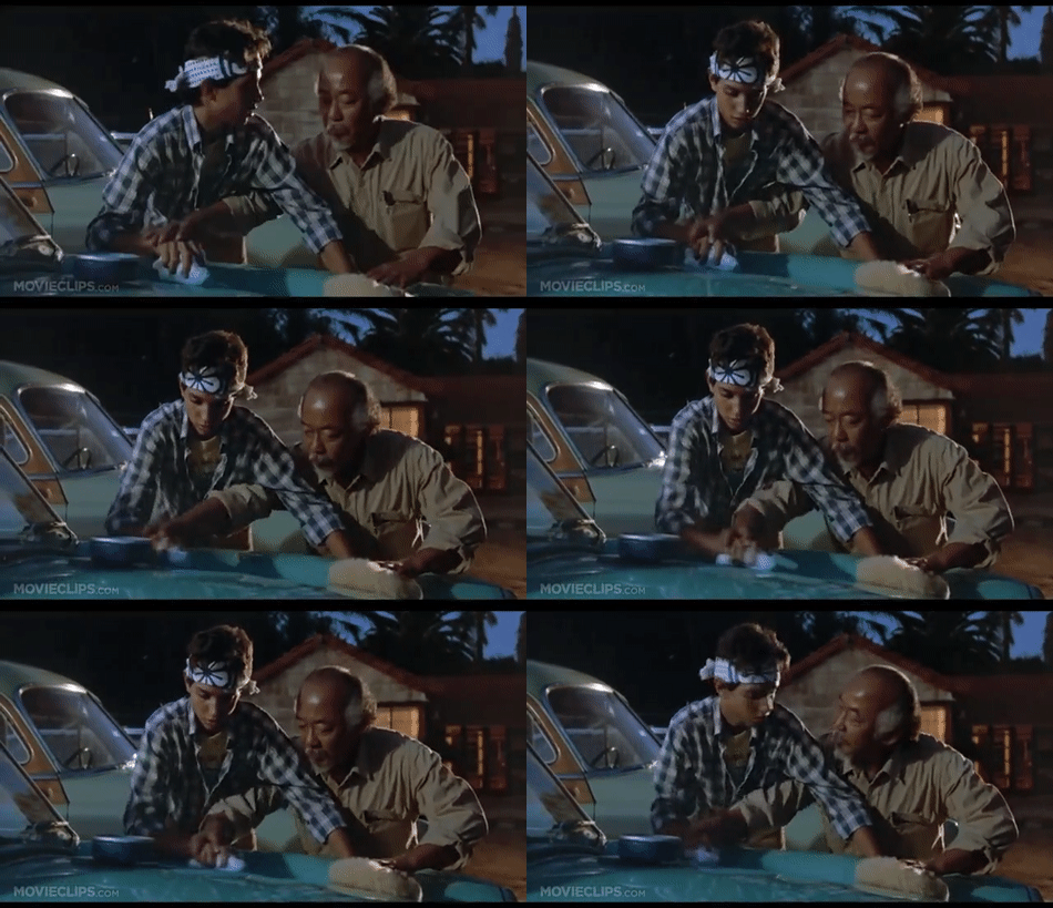] ] ] .hidden[ .grid[ .kol-6-12[ $$\begin{aligned} \text{Mr. Miyagi} &= \text{Deep Learning Practitioner} \\\\ \text{Daniel LaRusso} &= \text{ConvNet}\end{aligned}$$ ] .kol-6-12[ $$\begin{aligned}\text{daily chores} &= \text{pretext tasks} \\\\ \text{learning karate} &= \text{downstream task}\end{aligned}$$ ] ] ] --- class: middle, black-slide ## .center[Stage 1: Train .italic[muscle memory] on pretext tasks] .grid[ .kol-4-12[ .center.width-100[] ] .kol-4-12[ .center.width-100[] ] .kol-4-12[ .center.width-100[] ] ] .grid[ .kol-6-12[ $$\begin{aligned} \text{Mr. Miyagi} &= \text{Deep Learning Practitioner} \\\\ \text{Daniel LaRusso} &= \text{ConvNet}\end{aligned}$$ ] .kol-6-12[ $$\begin{aligned}\text{daily chores} &= \text{pretext tasks} \\\\ \text{learning karate} &= \text{downstream task}\end{aligned}$$ ] ] --- class: middle, black-slide ## .center[Stage 2: Fine-tune skills rapidly] .center.width-60[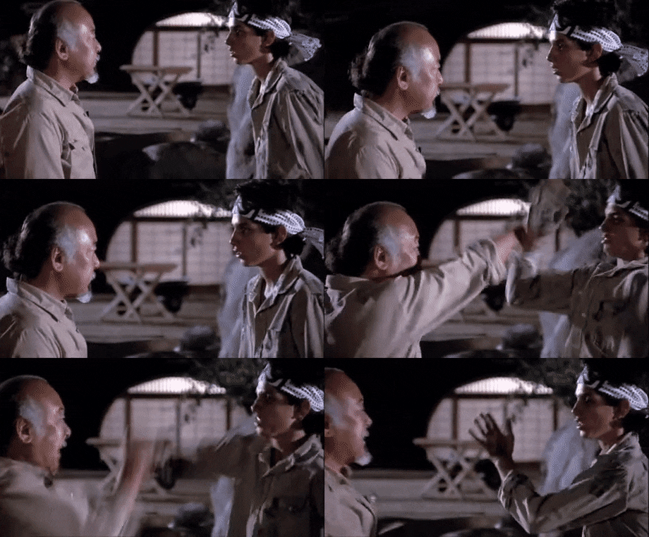] --- class: middle, black-slide <!-- ## .center[Stage 2: Fine-tune skills rapidly] --> .center.width-60[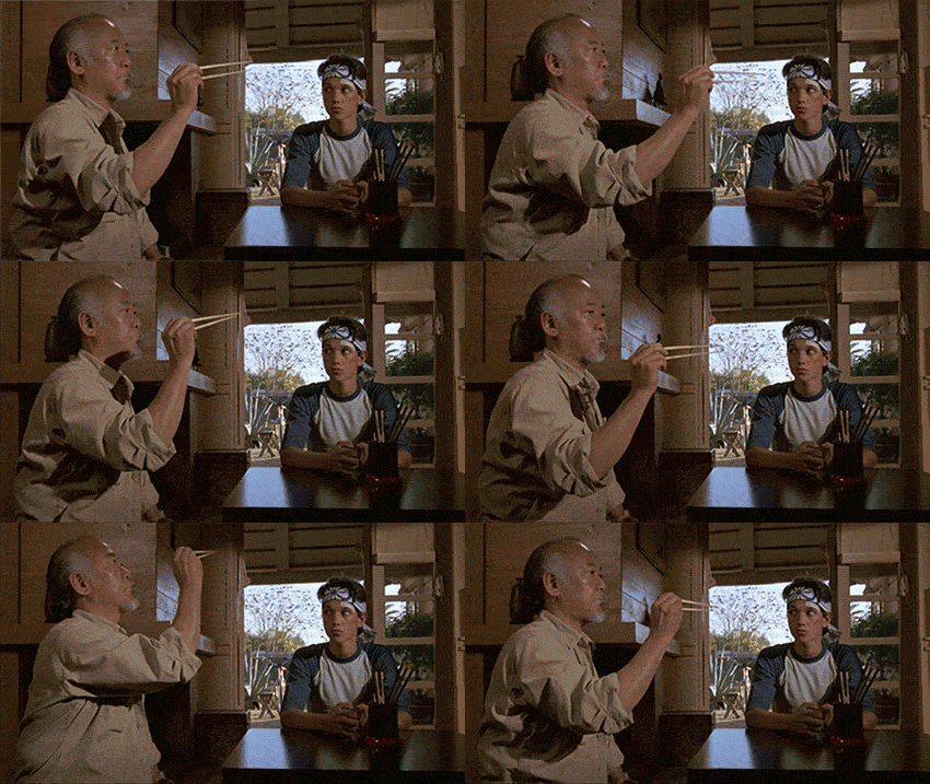] <!-- .caption[Mr. Myiagi during Stage 1] --> $$\text{Mr. Miyagi during Stage 1} = \text{catching up on ArXiv papers}$$ --- class: middle, center .Q[.big[Is this actually useful in practice?]] <!-- --- class: middle .grid[ .kol-6-12[ .center.width-100[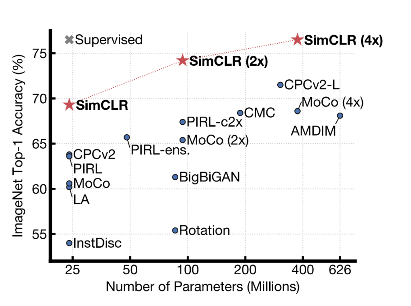] .caption[ImageNet Top-1 accuracy of linear classifiers trained on representations learned with different self-supervised methods (pretrained on ImageNet). Gray cross indicates supervised ResNet-50.] ] .kol-6-12[ <br/><br/><br/><br/><br/> The performance on linear classifiers on ImageNet has accelerated strongly in the past year closing the gap w.r.t. supervised methods ] ] .citation[T. Chen et al., A Simple Framework for Contrastive Learning of Visual Representations, ArXiv 2020 ] --> --- class: middle ## .center[Transfer learning - object detection] .grid[ .kol-6-12[ .center.width-90[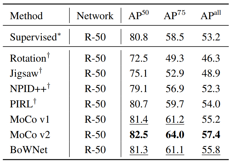] .caption[Object detection with Faster R-CNN fine-tuned on VOC $\texttt{trainval07+12}$ and evaluated on $\texttt{test07}$. Networks are pre-trained with self-supervision on ImageNet.] ] .kol-6-12[ <br><br><br> <br> - Self-supervised methods are starting to outperform supervised methods - This is a __key milestone for self-supervised methods__ as they are finally showing their effectiveness to more complex downstream tasks. ] ] .citation[S. Gidaris et al., Learning Representations by Predicting Bags of Visual Words, CVPR 2020] <!-- --- class: middle .big.italic.purple[".bold[Unsupervised learning:] Think hard about the model, use whatever data fits.] .big.italic.purple[.bold[Self-supervised learning:] Think hard about the data, use whatever model fits."] .bold.pull-right[Misha Denil] <br/> <br/> .center.width-30[] --> <!-- --- class: middle, center .highlight[ # Scope of this tutorial ] --> --- class: middle Loosely speaking, multiple old and new approaches could fit, at least partially, the definition of self-supervised learning: - input reconstruction: .cites[[Hinton and Salakhutdinov (2006); Vincent et al. (2008)]] - training with paired signals: .cites[[V. De Sa (1994); Arandjelovic and Zisserman (2017); C. Godard et al. (2017)]] - hiding data from the networks: .cites[[Doersch et al. (2015); Zhang et el. (2017)]] - instance discrimination: .cites[[Dosovitskiy et al. (2014); van der Ooord et al. (2018)]] - etc. <br/> <br/> .citation[G. Hinton and R. Salakhutdinov, Reducing the Dimensionality of Data with Neural Networks, Science 2006 <br/> P.Vincent et al.,Extracting and Composing Robust Features with Denoising Autoencoders, ICML 2008 <br/> V. De Sa, Learning classification from unlabelled data, NeurIPS 1994 <br/> R. Arandjelovic and A. Zisserman, Look, Listen and Learn, ICCV 2017 <br/> C. Godard et al., Unsupervised Monocular Depth Estimation with Left-Right Consistency, CVPR 2017 <br/> R. Zhang et al., Split-Brain Autoencoders: Unsupervised Learning by Cross-Channel Prediction, CVPR 2017 <br/> C. Doersch et al., Unsupervised Visual Representation Learning by Context Prediction, ICCV 2015 <br/> A. Dosovitskiy et al., Discriminative Unsupervised Feature Learning with Convolutional Neural Networks, NeurIPS 2015 <br/>A. van der Oord et al., Representation Learning with Contrastive Predictive Coding, ArXiv 2018 ] --- class: middle # .center[Scope] <!-- .center.big[In this tutorial, we **focus** on self-supervised methods that lead to *useful representations* (good baselines by themselves or amenable to improved performances after fine-tuning on a downstream task) *obtained through* the invention of *a pretext task and/or hiding a part of the original data* to the network.] --> .center.big[In this tutorial, we **focus** on self-supervised methods that lead <br/> to *useful representations*, obtained through the invention of *a pretext task* and/or *by hiding a part of the original data* to the network.] --- class: middle, center # 2. A tour of pretext tasks for Self-Supervised Learning <!-- .bigg.highlight[Relja] --> --- layout: false class: end-slide, center count: false .bigger[Handing the mic to Relja ...] --- layout: true .center.footer[Andrei BURSUC and Relja ARANDJELOVIĆ | Self-Supervised Learning] --- class: middle, center # 3. Practical considerations <!-- .bigg.highlight[Relja & Andrei] --> --- class: middle # Practical considerations ## Noise Contrastive Estimation --- class: middle Let $x \in \mathcal{X}$ be input data and $y \in \\{1, \dots, L\\}$ and $f\_{\theta}(\cdot):\mathcal{X}\rightarrow\mathbb{R}^D$ a network generating an embedding vector $f\_{\theta}(x)$. <!-- We use $x^{+}$ and $\\{x^{i}\\}$ to denote a positive sample and set of negative examples for $x$. --> We denote: - $q=f\_{\theta}(x)$ (*query*) - $\\{x^{i}\\}$ a set of samples from $\mathcal{X}$. - $k\_{i} = f\_{\theta}(x^{i})$ the embeddings of $\\{x^{i}\\}$ as keys (*representations*) --- class: middle ## Parametric Classifier - We are interested in instance discrimination, i.e. recognizing a particular query sample - We can formulate the instance-level classification objective using the softmax criterion - We consider each neuron from the last layer as a class-level weight vector $w\_{i}$ (with $b = 0$), i.e. _class prototype_ $$\mathcal{L}\_{\text{softmax}} (q, c(q)) = - \log\frac{\exp(q^\top w\_{c(q)})}{ \sum\_{c\in C}\exp(q^\top w\_{c})}$$ where: - $C$ is the number of classes - $c(q)$ is the class index of $q$ <!-- $$P ( j | q ) = \frac{\exp(q \cdot w\_j)}{ \sum\_{i=1}^{N}\exp(q \cdot w\_{i})}$$ --> .citation[Z. Wu et al., Unsupervised Feature Learning via Non-Parametric Instance Discrimination, CVPR 2018] --- class: middle ## Non-Parametric Classifier - Using $w\_i$ as class prototype prevents explicit comparison between instances, i.e. individual samples - We can use instead a _non-parametric_ variant that replaces $q^\top w\_j$ with $q^\top k\_i$ $$\mathcal{L}\_{\text{non-param-softmax}}(q) = - \log \frac{\exp(q^\top k\_q )}{ \sum\_{i \in N}\exp(q ^\top k\_{i})}$$ where: - $N$ is the number of training samples - $k\_q \in \\{ k\_i\\}$ is the key of a positive sample for $q$ .citation[Z. Wu et al., Unsupervised Feature Learning via Non-Parametric Instance Discrimination, CVPR 2018] --- count: false class: middle ## Non-Parametric Classifier - Using $w\_i$ as class prototype prevents explicit comparison between instances, i.e. individual samples - We can use instead a _non-parametric_ variant that replaces $q^\top w\_j$ with $q^\top k\_i$ $$\mathcal{L}\_{\text{softmax}} (q, c(q)) = - \log\frac{\exp(q^\top w\_{c(q)})}{ \sum\_{c\in C}\exp(q^\top w\_{c})} \longrightarrow \mathcal{L}\_{\text{non-param-softmax}}(q) = - \log \frac{\exp(q^\top k\_q )}{ \sum\_{i \in N}\exp(q ^\top k\_{i})}$$ where: - $N$ is the number of training samples - $k\_q \in \\{ k\_i\\}$ is the key of a positive sample for $q$ .citation[Z. Wu et al., Unsupervised Feature Learning via Non-Parametric Instance Discrimination, CVPR 2018] --- class: middle ## Non-Parametric Classifier .center.width-60[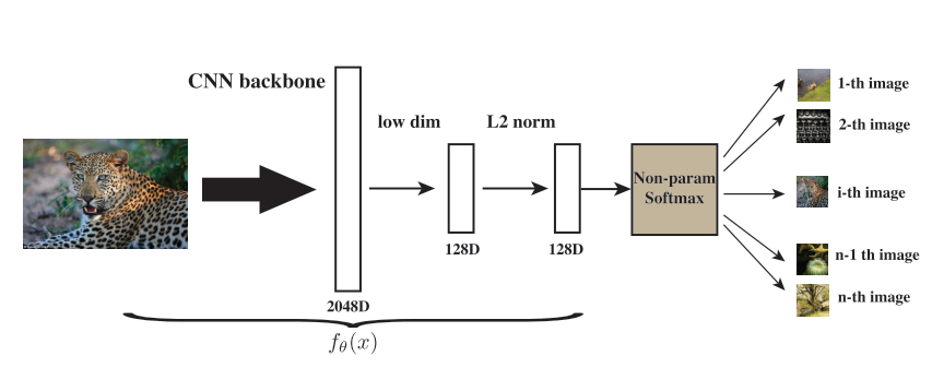] .caption[Self-supervised learning as image instance-level discrimination] $$ \mathcal{L}\_{\text{non-param-softmax}}(q) = - \log \frac{\exp(q^\top k\_q )}{ \sum\_{i \in N}\exp(q ^\top k\_{i})}$$ The learning objective focuses now entirely on feature representation, instead of class-specific representations .citation[Z. Wu et al., Unsupervised Feature Learning via Non-Parametric Instance Discrimination, CVPR 2018] --- class: middle ## Noise-Contrastive Estimation (NCE) - Computing the non-parametric softmax is expensive when the number of classes $N$ is very large, e.g. millions - Popular solutions: NCE, hierarchical softmax .hidden[ - .bold[NCE:] cast the multi-class classification into a set of binary classification problems, each discriminating between __data samples (positives)__ and __noise samples (negatives)__. $$\mathcal{L}\_{\text{NCE}}(q) = - \log \frac{\exp(q^\top k\_{q} )}{ Z\_q}$$ - The denominator $Z\_q$ is treated as constant and estimated via Monte Carlo approximation $$Z\_q = \sum\_{i \in N}\exp(q^\top k\_{i}) \simeq \frac{N}{K}\sum\_{j \in K}\exp(q^\top k\_{j})$$ where $K$ is the number Monte Carlo samples ] .citation[Z. Wu et al., Unsupervised Feature Learning via Non-Parametric Instance Discrimination, CVPR 2018<br/>M. Gutmann and A. Hyvarinen, Noise-contrastive estimation: A new estimation principle for unnormalized statistical models, AISTATS 2010] --- count: false class: middle ## Noise-Contrastive Estimation (NCE) - Computing the non-parametric softmax is expensive when the number of classes $N$ is very large, e.g. millions - Popular solutions: NCE, hierarchical softmax - .bold[NCE:] cast the multi-class classification into a set of binary classification problems, each discriminating between __data samples (positives)__ and __noise samples (negatives)__. $$\mathcal{L}\_{\text{NCE}}(q) = - \log \frac{\exp(q^\top k\_{q})}{ Z\_q}$$ - The denominator $Z\_q$ is treated as constant and estimated via Monte Carlo approximation $$Z\_q = \sum\_{i \in N}\exp(q^\top k\_{i}) \simeq \frac{N}{K}\sum\_{j \in K}\exp(q^\top k\_{j})$$ where $K$ is the number Monte Carlo samples .citation[Z. Wu et al., Unsupervised Feature Learning via Non-Parametric Instance Discrimination, CVPR 2018<br/>M. Gutmann and A. Hyvarinen, Noise-contrastive estimation: A new estimation principle for unnormalized statistical models, AISTATS 2010] --- class: middle ## The InfoNCE loss .citet[van der Oord et al. (2018)] proposed a loss based on NCE called __InfoNCE__: <!--$$\mathcal{L}\_{\text{InfoNCE}}({q, k^{+}, \\{k^{-}\\}};\theta) = - \log \frac{\exp(q \cdot k^{+} / \tau)}{\exp(q \cdot k^{+} / \tau) + \sum\_{i=1}^{K}\exp(q \cdot k^{-}\_{i} / \tau)}$$--> $$\mathcal{L}\_{\text{InfoNCE}}(q) = - \log \frac{\exp(q^\top k\_{q})}{\sum\_{i \in K}\exp(q^\top k\_{i})}$$ .hidden[ - Connection to _mutual information maximization_ between the variable $q$ and $k\_{q}$: <!-- $$I(q;k^{+}) \geq \log{K} - \mathcal{L}\_{\text{InfoNCE}}({q, k^{+}, \\{k^{-}\\}}; \theta) $$ --> $$I(q;k\_{q}) \geq \log{K} - \mathcal{L}\_{\text{InfoNCE}}(q) $$ - Minimizing the objective $\mathcal{L}$, maximizes the lower bound on the mutual information $I(q;k\_{q})$ - The $\log K$ term suggests that using more negative samples can lead to an improved representation ] .citation[A. van der Oord et al., Representation learning with contrastive predictive coding, ArXiv 2018<br/>M. Gutmann and A. Hyvarinen, Noise-contrastive estimation: A new estimation principle for unnormalized statistical models, AISTATS 2010] --- count: false class: middle ## The InfoNCE loss .citet[van der Oord et al. (2018)] proposed a loss based on NCE called __InfoNCE__: <!--$$\mathcal{L}\_{\text{InfoNCE}}({q, k^{+}, \\{k^{-}\\}};\theta) = - \log \frac{\exp(q \cdot k^{+} / \tau)}{\exp(q \cdot k^{+} / \tau) + \sum\_{i=1}^{K}\exp(q \cdot k^{-}\_{i} / \tau)}$$--> $$\mathcal{L}\_{\text{InfoNCE}}(q) = - \log \frac{\exp(q^\top k\_{q})}{\sum\_{i \in K}\exp(q^\top k\_{i})}$$ - Connection to _mutual information maximization_ between the variable $q$ and $k\_{q}$: <!-- $$I(q;k^{+}) \geq \log{K} - \mathcal{L}\_{\text{InfoNCE}}({q, k^{+}, \\{k^{-}\\}}; \theta) $$ --> $$I(q;k\_{q}) \geq \log{K} - \mathcal{L}\_{\text{InfoNCE}}(q) $$ - Minimizing the objective $\mathcal{L}$, maximizes the lower bound on the mutual information $I(q;k\_{q})$ - The $\log K$ term suggests that using more negative samples can lead to an improved representation .citation[A. van der Oord et al., Representation learning with contrastive predictive coding, ArXiv 2018<br/>M. Gutmann and A. Hyvarinen, Noise-contrastive estimation: A new estimation principle for unnormalized statistical models, AISTATS 2010] --- class: middle # Practical considerations ## Noise Contrastive Estimation - The Metric Learning perspective --- class: middle .center.width-65[] .caption[Deep metric learning with (left) triplet loss and (right) $(N+1)$-tuplet loss. <br/>$(N+1)$-tuplet loss pushes $N-1$ negative examples all at once.] Similar findings have been reached when studying this problem from a *metric learning perspective* by .citet[Sohn (2016)]. Their method that generalizes *triplet-loss* with **N-pair loss**, exploits multiple negatives for each query and has been shown to improve convergence speed and performance. .citation[K. Sohn, Improved Deep Metric Learning with Multi-class N-pair Loss Objective, NeurIPS 2016] ??? Embedding vectors $f$ of deep networks are trained to satisfy the constraints of each loss. Triplet loss pulls positive example while pushing one negative example at a time. On the other hand, $(N+1)$-tuplet loss pushes $N-1$ negative examples all at once, based on their similarity to the input example. --- class: middle - Contrastive loss (pair-wise) .cites[[Chopra et al. (2005), Hadsell et al. (2006)]] $$\mathcal{L}\_{\text{contrastive}}(q, k\_i) = \boldsymbol{1}\\{y\_q = y\_i\\} \\| q - k\_i\\|^{2}\_{2} +\boldsymbol{1}\\{y\_q =\not y\_i\\} \max(0, m - \\| q - k\_i\\|^{2}\_{2} )$$ where $m$ is the margin parameter - Triplet loss .cites[[M. Schultz and T. Joachim (2004); K. Weinberger et al. (2006); Schroff et al. (2015)]] $$\mathcal{L}\_{\text{triplet}}(q, k\_{q}, k\_{i}) = \max(0, \\| q - k\_{q}\\|^{2}\_{2} - \\| q - k\_{i}\\|^{2}\_{2} + m )$$ .hidden[ - N-pair loss .cites[[Sohn (2016)]] $$\mathcal{L}\_{\text{N-pair}}(q, k\_{q}, \\{k\_i\\}\_{i \in N}) = \log ( 1 +\sum\_{i=1}^{N-1}\exp(q^\top k\_{i} - q^\top k\_{q})$$ ] .hidden[ - InfoNCE loss .cites[[van der Ooord (2018)]] $$\mathcal{L}\_{\text{InfoNCE}}(q) = - \log \frac{\exp(q^\top k\_{q} )}{\sum\_{i \in K}\exp(q^\top k\_{i} ))}$$ <br/> ] .citation[S. Chopra et al., Learning a similarity metric discriminatively, with application to face verification, CVPR 2005; R. Hadsell et al., Dimensionality reduction by learning an invariant mapping, CVPR 2006; K. Weinberger et al., Distance metric learning for large margin nearest neighbor classification, NeurIPS 2006; M. Schultz and T. Joachims, Learning a distance metric from relative comparisons, NeurIPS 2004; F. Schroff et al., FaceNet: A unified embedding for face recognition and clustering, CVPR 2015; K. Sohn, Improved deep metric learning with multi-class N-pair loss objective, NeurIPS 2016 ] --- count: false class: middle - Contrastive loss (pair-wise) .cites[[Chopra et al. (2005), Hadsell et al. (2006)]] $$\mathcal{L}\_{\text{contrastive}}(q, k\_i) = \boldsymbol{1}\\{y\_q = y\_i\\} \\| q - k\_i\\|^{2}\_{2} +\boldsymbol{1}\\{y\_q =\not y\_i\\} \max(0, m - \\| q - k\_i\\|^{2}\_{2} )$$ where $m$ is the margin parameter - Triplet loss .cites[[M. Schultz and T. Joachim (2004); K. Weinberger et al. (2006); Schroff et al. (2015)]] $$\mathcal{L}\_{\text{triplet}}(q, k\_{q}, k\_{i}) = \max(0, \\| q - k\_{q}\\|^{2}\_{2} - \\| q - k\_{i}\\|^{2}\_{2} + m )$$ - N-pair loss .cites[[Sohn (2016)]] $$\mathcal{L}\_{\text{N-pair}}(q, k\_{q}, \\{k\_i\\}\_{i \in N}) = \log ( 1 +\sum\_{i=1}^{N-1}\exp(q^\top k\_{i} - q^\top k\_{q}))$$ .hidden[ - infoNCE loss .cites[[van der Ooord (2018)]] $$\mathcal{L}\_{\text{InfoNCE}}(q) = - \log \frac{\exp(q^\top k\_{q} )}{\sum\_{i \in K}\exp(q^\top k\_{i} )}$$ ] <br/> .citation[S. Chopra et al., Learning a similarity metric discriminatively, with application to face verification, CVPR 2005; R. Hadsell et al., Dimensionality reduction by learning an invariant mapping, CVPR 2006; K. Weinberger et al., Distance metric learning for large margin nearest neighbor classification, NeurIPS 2006; M. Schultz and T. Joachims, Learning a distance metric from relative comparisons, NeurIPS 2004; F. Schroff et al., FaceNet: A unified embedding for face recognition and clustering, CVPR 2015; K. Sohn, Improved deep metric learning with multi-class N-pair loss objective, NeurIPS 2016 ] --- count: false class: middle - Contrastive loss (pair-wise) .cites[[Chopra et al. (2005), Hadsell et al. (2006)]] $$\mathcal{L}\_{\text{contrastive}}(q, k\_i) = \boldsymbol{1}\\{y\_q = y\_i\\} \\| q - k\_i\\|^{2}\_{2} +\boldsymbol{1}\\{y\_q =\not y\_i\\} \max(0, m - \\| q - k\_i\\|^{2}\_{2} )$$ where $m$ is the margin parameter - Triplet loss .cites[[M. Schultz and T. Joachim (2004); K. Weinberger et al. (2006); Schroff et al. (2015)]] $$\mathcal{L}\_{\text{triplet}}(q, k\_{q}, k\_{i}) = \max(0, \\| q - k\_{q}\\|^{2}\_{2} - \\| q - k\_{i}\\|^{2}\_{2} + m )$$ - N-pair loss .cites[[Sohn (2016)]] $$\mathcal{L}\_{\text{N-pair}}(q, k\_{q}, \\{k\_i\\}\_{i \in N}) = \log ( 1 +\sum\_{i=1}^{N-1}\exp(q^\top k\_{i} - q^\top k\_{q}))$$ - infoNCE loss .cites[[van der Ooord (2018)]] $$\mathcal{L}\_{\text{InfoNCE}}(q) = - \log \frac{\exp(q^\top k\_{q} )}{\sum\_{i \in K}\exp(q^\top k\_{i} )}$$ <br/> .citation[S. Chopra et al., Learning a similarity metric discriminatively, with application to face verification, CVPR 2005; R. Hadsell et al., Dimensionality reduction by learning an invariant mapping, CVPR 2006; K. Weinberger et al., Distance metric learning for large margin nearest neighbor classification, NeurIPS 2006; M. Schultz and T. Joachims, Learning a distance metric from relative comparisons, NeurIPS 2004; F. Schroff et al., FaceNet: A unified embedding for face recognition and clustering, CVPR 2015; K. Sohn, Improved deep metric learning with multi-class N-pair loss objective, NeurIPS 2016 ] --- class: middle .bigger[A key component in metric learning is related to negatives, in particular _hard negatives_.] .hidden.bigger[We have seen in InfoNCE that more negatives lead to improved representations.] .hidden.bigger[Bridging these two views can lead to a better understanding of contrastive learning and to transfering know-how from metric learning.] --- count: false class: middle .bigger[A key component in metric learning is related to negatives, in particular _hard negatives_.] .bigger[We have seen in InfoNCE that more negatives lead to improved representations.] .hidden.bigger[Bridging these two views can lead to a better understanding of contrastive learning and to transfering know-how from metric learning.] --- count: false class: middle .bigger[A key component in metric learning is related to negatives, in particular _hard negatives_.] .bigger[We have seen in InfoNCE that more negatives lead to improved representations.] .bigger[Bridging these two views can lead to a better understanding of contrastive learning and to transfering know-how from metric learning.] --- class: middle .bigger[In recent literature InfoNCE is the most popular and, so far, the best performing loss for contrastive self-supervised learning.] .bigger[We will outline a few strategies to make it work effectively. ] --- class: middle # Practical considerations ## Dealing with negative samples --- class: middle .center.bigger[Multiple works have observed the influence of negative samples and proposed different heuristics to increase their number.] .grid[ .kol-4-12[ .caption[CMC .cites[[Tian et al. (2019)]]] .center.width-105[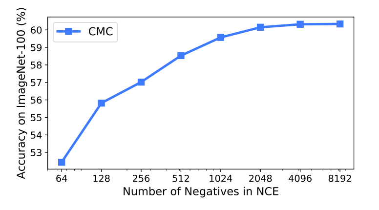] ] .kol-4-12[ .caption[MoCo .cites[[He et al. (2020)]]] .center.width-105[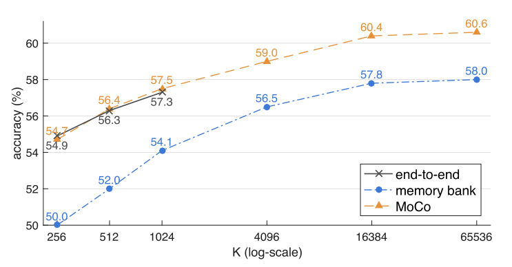] ] .kol-4-12[ .caption[PiRL .cites[[Misra and van der Maaten (2020)]]] .center.width-105[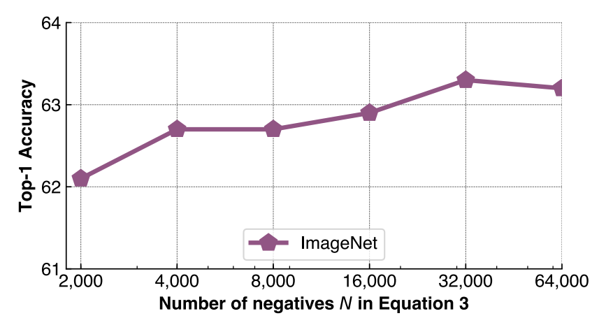] ] ] .citation[Y. Tian et al., Contrastive Multiview Coding, ArXiv 2019 <br/>K. He et al., Momentum Contrast for Unsupervised Visual Representation Learning, CVPR 2020<br/> I. Misra and L. van der Maaten, Self-Supervised Learning of Pretext-Invariant Representations, CVPR 2020] --- class: middle .center[## InfoNCE loss might not work at all down from a certain number of negatives.] .center.width-50[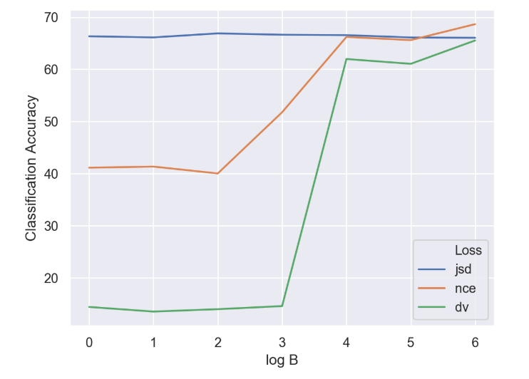] .caption[Classification accuracies for DeepInfoMax on CIFAR10. Accuracies shown averaged over the last 100 epochs for the _InfoNCE_, _JSD_, and _DV DIM_ losses. x-axis is log base-2 of the number of negative samples (0 mean one negative sample per positive sample).] .citation[R.D. Hjelm et al.,Learning deep representations by mutual information estimation and maximization, ICLR 2019] --- # End-to-End training .grid[ .kol-4-12[ .center.width-115[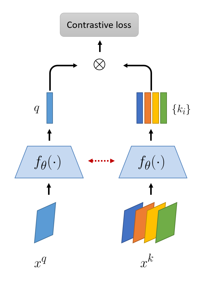] <!-- <img src="images/pairwise-1.png" style="width: 375px;" /> --> ] .kol-1-12[] .kol-7-12[ <br/> - Shared encoder for queries and keys ] ] .citation[R. Hadsell et al., Dimensionality reduction by learning an invariant mapping, CVPR 2006; F. Schroff et al., FaceNet: A unified embedding for face recognition and clustering, CVPR 2015] --- count: false # End-to-End training .grid[ .kol-4-12[ .center.width-115[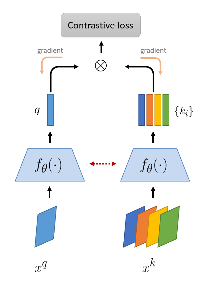] <!-- <img src="images/pairwise-2.png" style="width: 375px;" /> --> ] .kol-1-12[] .kol-7-12[ <br/> - Shared encoder for queries and keys - The encoder is updated by backpropagation through all samples ] ] .citation[R. Hadsell et al., Dimensionality reduction by learning an invariant mapping, CVPR 2006; F. Schroff et al., FaceNet: A unified embedding for face recognition and clustering, CVPR 2015] --- count: false # End-to-End training .grid[ .kol-4-12[ .center.width-115[] <!-- <img src="images/pairwise-2.png" style="width: 375px;" /> --> ] .kol-1-12[] .kol-7-12[ <br/> - Shared encoder for queries and keys - The encoder is updated by backpropagation through all samples .bigger.green[Pros] - Consistent $q$ and $\\{k\_{i}\\}$ ] ] .citation[R. Hadsell et al., Dimensionality reduction by learning an invariant mapping, CVPR 2006; F. Schroff et al., FaceNet: A unified embedding for face recognition and clustering, CVPR 2015] --- count: false # End-to-End training .grid[ .kol-4-12[ .center.width-115[] <!-- <img src="images/pairwise-2.png" style="width: 375px;" /> --> ] .kol-1-12[] .kol-7-12[ <br/> - Shared encoder for queries and keys - The encoder is updated by backpropagation through all samples .bigger.green[Pros] - Consistent $q$ and $\\{k\_{i}\\}$ .bigger.red[Cons] - The amount of negatives limited by GPU memory ] ] .citation[R. Hadsell et al., Dimensionality reduction by learning an invariant mapping, CVPR 2006; F. Schroff et al., FaceNet: A unified embedding for face recognition and clustering, CVPR 2015] --- # End-to-End training .grid[ .kol-4-12[ .center.width-115[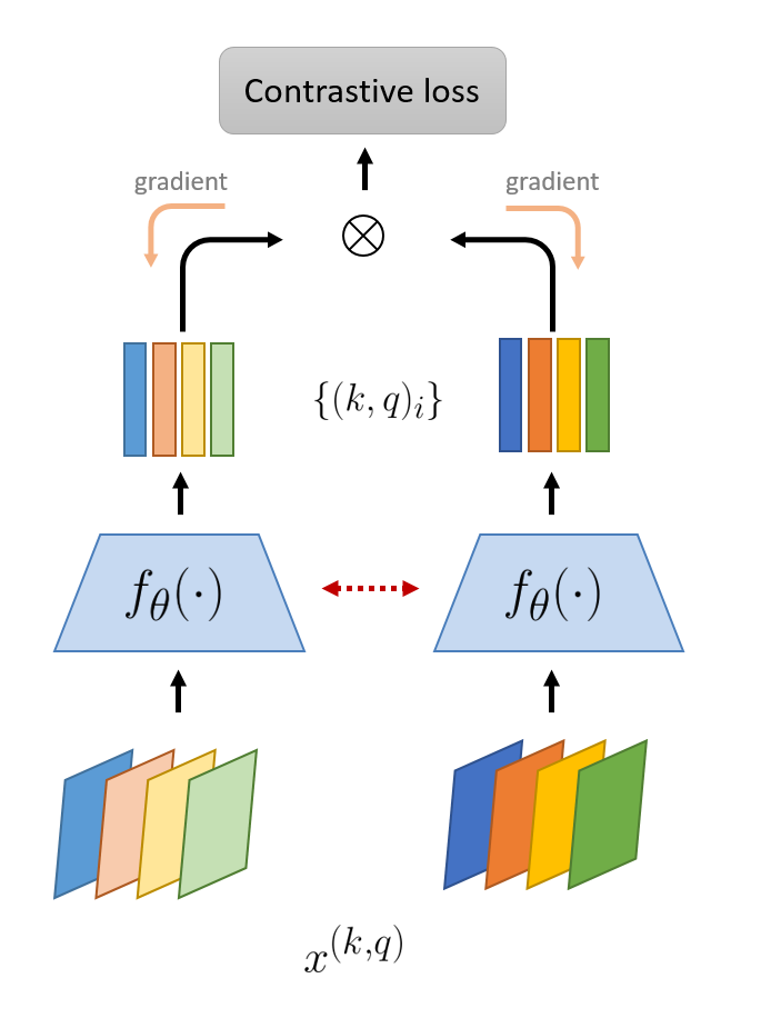] <!-- <img src="images/pairwise-3.png" style="width: 375px;" /> --> ] .kol-1-12[] .kol-7-12[ <br/> - Rely on large mini-batches ($2k-8k$ samples) to ensure plenty of negatives, e.g. $16382$ negatives from a batch of $8192$, i.e. $2(N-1)$ negatives - The loss is computed across all positive pairs in a mini-batch ] ] .citation[T. Chen et al., A Simple Framework for Contrastive Learning of Visual Representations, ArXiv 2020 ] ??? - _SimCLR_ .cites[[Chen et al. (2010)]] also takes an end-to-end approach --- count: false # End-to-End training .grid[ .kol-4-12[ .center.width-115[] <!-- <img src="images/pairwise-3.png" style="width: 375px;" /> --> ] .kol-1-12[] .kol-7-12[ <br/> - Rely on large mini-batches ($2k-8k$ samples) to ensure plenty of negatives, e.g. $16382$ negatives from a batch of $8192$, i.e. $2(N-1)$ negatives - The loss is computed across all positive pairs in a mini-batch .bigger.green[Pros] - Lots of negatives ] ] .citation[T. Chen et al., A Simple Framework for Contrastive Learning of Visual Representations, ArXiv 2020 ] --- count: false # End-to-End training .grid[ .kol-4-12[ .center.width-115[] <!-- <img src="images/pairwise-3.png" style="width: 375px;" /> --> ] .kol-1-12[] .kol-7-12[ <br/> - Rely on large mini-batches ($2k-8k$ samples) to ensure plenty of negatives, e.g. $16382$ negatives from a batch of $8192$, i.e. $2(N-1)$ negatives - The loss is computed across all positive pairs in a mini-batch .bigger.green[Pros] - Lots of negatives .bigger.red[Cons] - Lots of GPUs/TPUs ] ] .citation[T. Chen et al., A Simple Framework for Contrastive Learning of Visual Representations, ArXiv 2020 ] --- # Memory bank .grid[ .kol-4-12[ .center.width-115[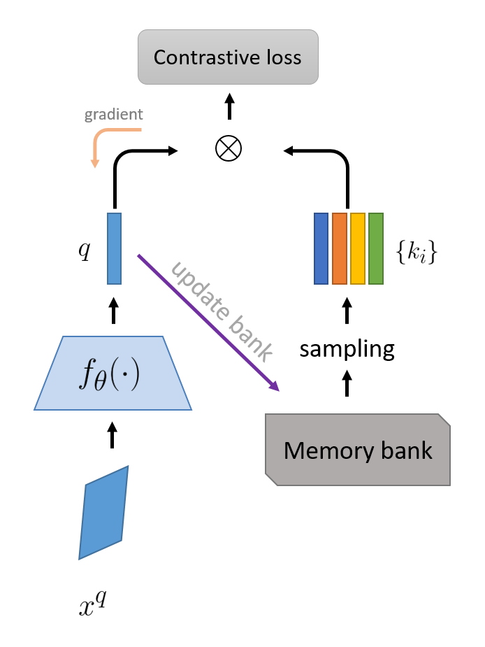] <!-- <img src="images/memory-bank-1.png" style="width: 375px;" /> --> ] .kol-1-12[] .kol-7-12[ <br/> - Keys are randomly sampled from a _memory bank_ of cached features - The memory bank contains features or all images in the dataset - There is no backpropagation through the memory bank - Keys are updated via exponential moving average .hidden[ .bigger.green[Pros] - Many negatives ($K = 65536$) while GPU memory efficient ] ] ] .citation[Z. Wu et al., Unsupervised Feature Learning via Non-Parametric Instance Disc., CVPR 2018; I. Misra et al., Self-Sup. Learning of Pretext-Invariant Representations, CVPR 2020 ] --- count:false # Memory bank .grid[ .kol-4-12[ .center.width-115[] <!-- <img src="images/memory-bank-1.png" style="width: 375px;" /> --> ] .kol-1-12[] .kol-7-12[ <br/> - Keys are randomly sampled from a _memory bank_ of cached features - The memory bank contains features or all images in the dataset - There is no backpropagation through the memory bank - Keys are updated via exponential moving average .bigger.green[Pros] - Many negatives ($K = 65536$) while GPU memory efficient ] ] .citation[Z. Wu et al., Unsupervised Feature Learning via Non-Parametric Instance Disc., CVPR 2018; I. Misra et al., Self-Sup. Learning of Pretext-Invariant Representations, CVPR 2020 ] --- count:false # Memory bank .grid[ .kol-4-12[ .center.width-115[] <!-- <img src="images/memory-bank-1.png" style="width: 375px;" /> --> ] .kol-1-12[] .kol-7-12[ <br/> - Keys are randomly sampled from a _memory bank_ of cached features - The memory bank contains features or all images in the dataset - There is no backpropagation through the memory bank - Keys are updated via exponential moving average .bigger.green[Pros] - Many negatives ($K = 65536$) while GPU memory efficient .bigger.red[Cons] - Keys are .italic["older" ] than queries ] ] .citation[Z. Wu et al., Unsupervised Feature Learning via Non-Parametric Instance Disc., CVPR 2018; I. Misra et al., Self-Sup. Learning of Pretext-Invariant Representations, CVPR 2020 ] ??? - Sampled features correspond to encoders at different steps in the past epoch and are less consistent --- # Momentum encoder .grid[ .kol-4-12[ .center.width-115[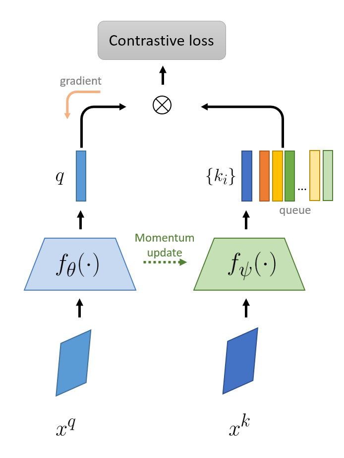] <!-- <img src="images/moco-1.png" style="width: 375px;" /> --> ] .kol-1-12[] .kol-7-12[ - _Momentum encoder_ relies on a memory-bank with a different update scheme - The encoder $f\_{\psi}(\cdot)$ is updated instead of the keys themselves - New samples are continuously added to the memory bank - The momentum encoder $f\_{\psi}(\cdot)$ is slowly pursuing $f\_{\theta}(\cdot)$ via exponential moving average, i.e. momentum, update: $$\psi \leftarrow m \psi + (1-m)\theta $$ ] ] .citation[K. He et al., Momentum Contrast for Unsupervised Visual Representation Learning, CVPR 2020] --- count: false # Momentum encoder .grid[ .kol-4-12[ .center.width-115[] <!-- <img src="images/moco-1.png" style="width: 375px;" /> --> ] .kol-1-12[] .kol-7-12[ - _Momentum encoder_ relies on a memory-bank with a different update scheme - The encoder $f\_{\psi}(\cdot)$ is updated instead of the keys themselves - New samples are continuously added to the memory bank - The momentum encoder $f\_{\psi}(\cdot)$ is slowly pursuing $f\_{\theta}(\cdot)$ via exponential moving average, i.e. momentum, update: $$\psi \leftarrow m \psi + (1-m)\theta $$ ```py q = f_q.forward(x_q) # queries: NxC k = f_k.forward(x_k) # keys: NxC k = k.detach() # no gradient to keys ... # SGD update: query network loss.backward() update(f_q.params) # momentum update: key network f_k.params = m*f_k.params+(1-m)*f_q.params ``` ] ] .citation[K. He et al., Momentum Contrast for Unsupervised Visual Representation Learning, CVPR 2020] --- count: false # Momentum encoder .grid[ .kol-4-12[ .center.width-115[] <!-- <img src="images/moco-1.png" style="width: 375px;" /> --> ] .kol-1-12[] .kol-7-12[ - _Momentum encoder_ relies on a memory-bank with a different update scheme - The encoder $f\_{\psi}(\cdot)$ is updated instead of the keys themselves - New samples are continuously added to the memory bank - The momentum encoder $f\_{\psi}(\cdot)$ is slowly pursuing $f\_{\theta}(\cdot)$ via exponential moving average, i.e. momentum, update: $$\psi \leftarrow m \psi + (1-m)\theta $$ ```py q = f_q.forward(x_q) # queries: NxC k = f_k.forward(x_k) # keys: NxC k = k.detach() # no gradient to keys ... # SGD update: query network loss.backward() update(f_q.params) # momentum update: key network *f_k.params = m*f_k.params+(1-m)*f_q.params ``` ] ] .citation[K. He et al., Momentum Contrast for Unsupervised Visual Representation Learning, CVPR 2020] --- count: false # Momentum encoder .grid[ .kol-4-12[ .center.width-115[] <!-- <img src="images/moco-1.png" style="width: 375px;" /> --> ] .kol-1-12[] .kol-7-12[ <br/><br/> .bigger.green[Pros] - Elegant and effective solution for large dictionaries .bigger.red[Cons] - Momentum requires tuning: $m \in [0.99, 0.9999]$ works well, while for $m \le 0.9$ accuracy drops considerably. - No backprop through the memory bank ] ] .citation[K. He et al., Momentum Contrast for Unsupervised Visual Representation Learning, CVPR 2020] --- class: middle # Practical considerations ## Output projection --- .grid[ .kol-4-12[ .center.width-115[] <!-- <img src="images/pairwise-3.png" style="width: 375px;" /> --> ] .kol-1-12[] .kol-7-12[ <br/><br/><br/><br/><br/> - Add a small neural network _projection head_ $g\_{\phi}(\cdot)$ right before contrastive loss ] ] .citation[T. Chen et al., A Simple Framework for Contrastive Learning of Visual Representations, ArXiv 2020 ] --- count: false .grid[ .kol-4-12[ .center.width-115[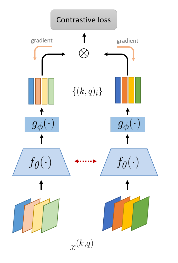] <!-- <img src="images/pairwise-4.png" style="width: 375px;" /> --> ] .kol-1-12[] .kol-7-12[ <br/><br/><br/><br/><br/> - Add a small neural network _projection head_ $g\_{\phi}(\cdot)$ right before contrastive loss - $g\_{\phi}(\cdot)$ can be a MLP with one hidden layer and ReLU - $g\_{\phi}(\cdot)$ is removed for the downstream task ] ] .citation[T. Chen et al., A Simple Framework for Contrastive Learning of Visual Representations, ArXiv 2020 ] --- # Output projection This cost-effective idea brings consist gains across methods ($+6-10\\%$) .grid[ .kol-6-12[ .center.width-100[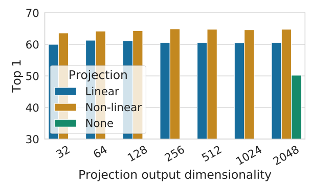] .caption[Linear evaluation of representations with different projection heads $g\_{\psi}(\cdot)$ and various output dimensions.] ] .kol-6-12[ ] ] .citation[T. Chen et al., A Simple Framework for Contrastive Learning of Visual Representations, ArXiv 2020 <br/> K. He et al., Improved Baselines with Momentum Contrastive Learning, ArXiv 2020] --- count: false # Output projection This cost-effective idea brings consist gains across methods ($+6-10\\%$) .grid[ .kol-6-12[ .center.width-100[] .caption[Linear evaluation of representations with different projection heads $g\_{\psi}(\cdot)$ and various output dimensions.] ] .kol-6-12[ <br/><br/><br/> .center.width-100[] .caption[ImageNet linear classification accuracy with MoCo v2] ] ] .citation[T. Chen et al., A Simple Framework for Contrastive Learning of Visual Representations, ArXiv 2020 <br/> K. He et al., Improved Baselines with Momentum Contrastive Learning, ArXiv 2020] --- class: middle .bigger[Due to loss of information induced by the contrastive loss, $g\_{\phi}(\cdot)$ can remove information that may be useful for the downstream taks, e.g. color, orientation of objects. ] <!-- This information is however preserved in $f\_{\theta}(\cdot)$. --> .center.width-55[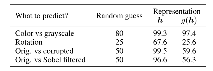] .caption[Accuracy of training additional MLPs on different representations to predict the transformation applied.] .citation[T. Chen et al., A Simple Framework for Contrastive Learning of Visual Representations, ArXiv 2020] --- class: middle # Practical considerations ## Hyperparameters --- class: middle .center.width-35[] .center.bigger[Recent contrastive methods require getting a few key ingredients to work properly.] .credit[Source: https://favpng.com/] --- <br/> ## Feature normalization - Without $\ell\_{2}$-normalization, the $\text{softmax}$ distribution can be made arbitrarily sharp by simply scaling all the features. --- count: false <br/> ## Feature normalization - Without $\ell\_{2}$-normalization, the $\text{softmax}$ distribution can be made arbitrarily sharp by simply scaling all the features. ## Temperature scaling - Mitigates peaky predictions from $\text{softmax}$ by increasing entropy <br/> $$\mathcal{L}\_{\text{InfoNCE}}(q) = - \log \frac{\exp(q^\top k\_{q} )}{\sum\_{i \in K}\exp(q^\top k\_{i} )} \longrightarrow \mathcal{L}\_{\text{InfoNCE}}(q) = - \log \frac{\exp(q^\top k\_{q} / \tau )}{\sum\_{i \in K}\exp(q^\top k\_{i} /\tau )} $$ .citation[G. Hinton et al., Distilling the knowledged in a neural network, ArXiv 2015<br/>T. Chen et al., A Simple Framework for Contrastive Learning of Visual Representations, ArXiv 2020] ??? - The temperature parameter $\tau$ controls the concentration level of the $\text{softmax}$ distribution --- count: false <br/> ## Feature normalization - Without $\ell\_{2}$-normalization, the $\text{softmax}$ distribution can be made arbitrarily sharp by simply scaling all the features. ## Temperature scaling - Mitigates peaky predictions from $\text{softmax}$ by increasing entropy .center.width-45[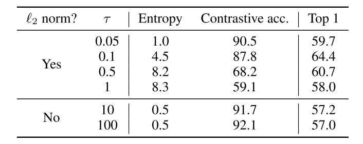] .caption[Linear evaluation for models trained with different choices of <br/> $\ell\_2$-normalization and temperature $\tau$.] .citation[G. Hinton et al., Distilling the knowledged in a neural network, ArXiv 2015<br/>T. Chen et al., A Simple Framework for Contrastive Learning of Visual Representations, ArXiv 2020] ??? - The temperature parameter $\tau$ controls the concentration level of the $\text{softmax}$ distribution --- count: false <br/> ## Feature normalization - Without $\ell\_{2}$-normalization, the $\text{softmax}$ distribution can be made arbitrarily sharp by simply scaling all the features. ## Temperature scaling - Mitigates peaky predictions from $\text{softmax}$ by increasing entropy ## Downstream hyperparameters - use specific hyperparameters for self-supervised method, e.g. larger learning rate, trainable BN layers .citation[G. Hinton et al., Distilling the knowledged in a neural network, ArXiv 2015<br/>T. Chen et al., A Simple Framework for Contrastive Learning of Visual Representations, ArXiv 2020 <br/>Y. Tian et al.Contrastive Multiview Coding, ArXiv 2019 <br/> K. He et al., Momentum Contrast for Unsupervised Visual Representation Learning, CVPR 2020] --- class: middle # Practical considerations ## Data augmentation --- class: middle .center.bigger[Data augmentation is known to be useful for recent self-supervised works. <br/>The rule of thumb was usually _.italic[whatever works well for supervised learning]_. ] --- class: middle .bigger[Impact of data augmentation tuning on self-supervised methods has been thoroughly studied only recently by .citet[Chen et al. (2020)]] .center.width-70[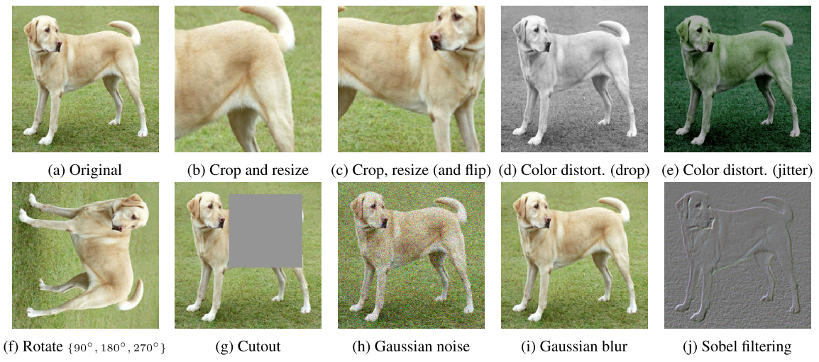] .caption[Typical data augmentation operators used for visual representation learning] .citation[T. Chen et al., A Simple Framework for Contrastive Learning of Visual Representations, ArXiv 2020] --- class: middle .grid[ .kol-6-12[ .center.width-100[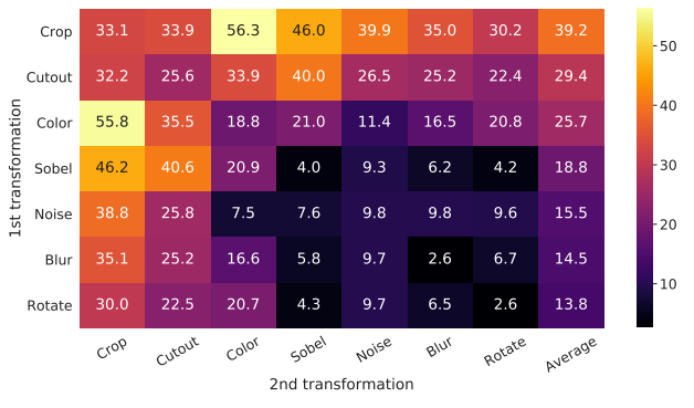] .caption[Linear evaluation (ImageNet top-1 accuracy) under individual or composition of data augmentations. ] ] .kol-6-12[ ] ] .citation[T. Chen et al., A Simple Framework for Contrastive Learning of Visual Representations, ArXiv 2020] ??? Diagonal entries correspond to single transformation, and off-diagonals correspond to composition of two transformations (applied sequentially). --- class: middle count: false .grid[ .kol-6-12[ .center.width-100[] .caption[Linear evaluation (ImageNet top-1 accuracy) under individual or composition of data augmentations. ] ] .kol-6-12[ <br/> - Composing augmentations makes the task harder and improves the quality of the representation - Contrastive learning needs stronger data augmentation than supervised learning - A well tuned augmentation strategy can lead to improvements of $3-4\\%$ alone ] ] .citation[T. Chen et al., A Simple Framework for Contrastive Learning of Visual Representations, ArXiv 2020] ??? - Diagonal entries correspond to single transformation, and off-diagonals correspond to composition of two transformations (applied sequentially). --- class: middle, center # 4. Evaluating Self-Supervised methods <!-- .bigg.highlight[Andrei] --> --- class: middle # Evaluating Self-Supervised methods ## Tasks and protocols --- class: middle .bigger[Self-supervised methods are evaluated on a battery of datasests and tasks .cites[[Goyal et al. (2019), <br/> Zhai et al. (2019)]]] .bigger[In most benchmarks the model is *pre-trained on ImageNet* on a pretext task and *subsequentely fine-tuned on other datasets* or protocols.] .citation[P. Goyal et al., Scaling and Benchmarking Self-Supervised Visual Representation Learning, ICCV 2019 <br/> X. Zhai et al., A Large-scale Study of Representation Learning with the Visual Task Adaptation Benchmark, ArXiv 2019] --- class: middle # Evaluation tasks <br/> ## Linear classification <br/> ## Few-shot learning <br/> ## Efficient learning <br/> ## Transfer learning --- # Linear classification .center.width-70[] - Simplest evaluation of the utility of learned representations: fit a linear classifier (FC layer, linear SVM) - .bold[Typical datasets:] + ImageNet + Places205 + Pascal VOC07 (image classification) + COCO14 (image classification) .citation[P. Goyal et al., Scaling and Benchmarking Self-Supervised Visual Representation Learning, ICCV 2019] --- # Linear classification .grid[ .kol-6-12[ .center.width-100[] .caption[ImageNet Top-1 accuracy of linear classifiers trained on representations learned with different self-supervised methods (pretrained on ImageNet). ] ] .kol-6-12[ <br><br> - The performance on this benchmark has accelerated strongly in the past year closing the gap w.r.t. supervised methods ] ] .citation[T. Chen et al., A Simple Framework for Contrastive Learning of Visual Representations, ArXiv 2020 ] --- count: false # Linear classification .grid[ .kol-6-12[ .center.width-100[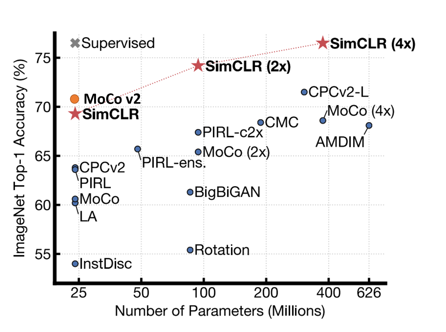] .caption[ImageNet Top-1 accuracy of linear classifiers trained on representations learned with different self-supervised methods (pretrained on ImageNet). ] ] .kol-6-12[ <br><br> - The performance on this benchmark has accelerated strongly in the past year closing the gap w.r.t. supervised methods - The main contributors: - _contrastive learning with more negatives_ - _output projection head_ - _better designed and stronger data augmentation_ - _longer training_ ] ] .citation[T. Chen et al., A Simple Framework for Contrastive Learning of Visual Representations, ArXiv 2020 ] --- class: middle ## .center[Linear classification on other datasets] .grid[ .kol-6-12[ .center.width-90[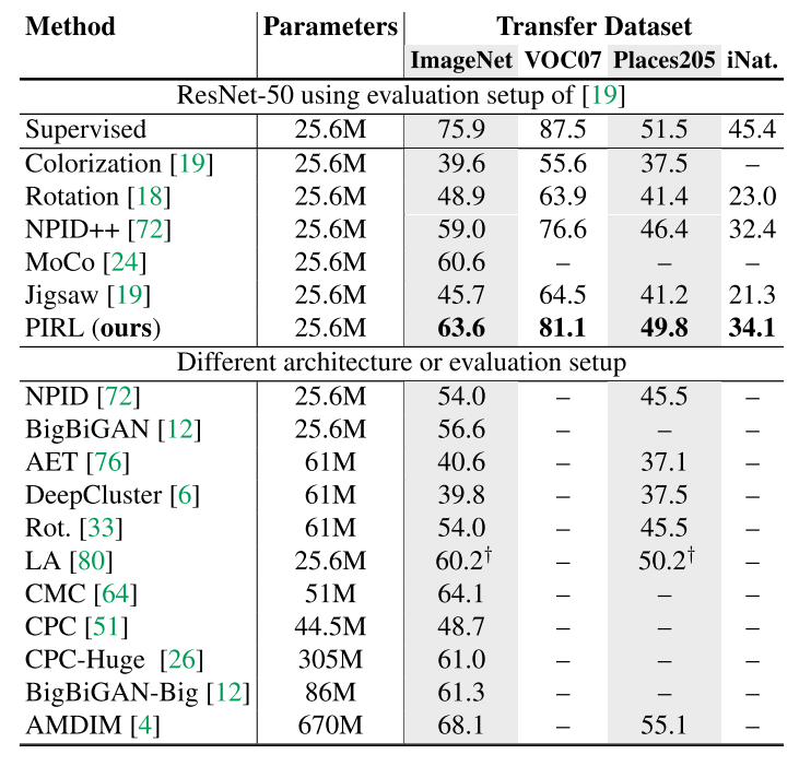] ] .kol-6-12[ <br><br><br><br><br> <br><br> .caption[Image classification performance on ImageNet, VOC07, Places205, and iNaturalist datasets. Linear classifiers are trained on image representations obtained by self-supervised learners that were pre-trained on ImageNet.] ] ] .citation[I. Misra and L. van der Maaten, Self-Supervised Learning of Pretext-Invariant Representations, CVPR 2020 ] ??? - The ranking of the methods usually remains unchanged for contrastive methods --- # Few-shot learning .center.width-70[] - Very similar goals of few-shot and self-supervised learning $\longrightarrow$ *.italic[Let's use same evaluation settings!]* - Thousands of small _train_-_test_ splits are proposed, leading to robust evaluation statistics. - .bold[Datasets:] miniImageNet .citation[S. Gidaris et al., Boosting Few-Shot Learning with Self-Supervision, ICCV 2019] ??? - The utility of learned representations can be also evaluated using the few-shot learning evaluation protocol - This comparison method could be more meaningful for assessing different self-supervised features --- # Few-shot learning .grid[ .kol-6-12[ <br><br> .center.width-100[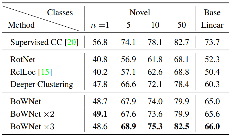] .caption[Average 5-way classification accuracies on the test set of MiniImageNet.] ] .kol-6-12[ <br><br><br><br><br> - Self-supervision reaches relatively competitive performance against the supervised .italic[Cosine Classifier] ] ] .citation[S. Gidaris et al., Learning Representations by Predicting Bags of Visual Words, CVPR 2020] --- # Efficient classification .center.width-70[] - Fine-tune pre-trained network on a subset of labels $1\\%-100\\%$ - .bold[Datasets:] ImageNet, VTAB .citation[X. Zhai et al., S4L: Self-Supervised Semi-Supervised Learning, ICCV 2019 <br/>X. Zhai et al., A Large-scale Study of Representation Learning with the Visual Task Adaptation Benchmark, ArXiv 2019 ] ??? - ImageNet is still the most popular choice, though new datasets are proposes now, e.g. VTAB benchmark --- # Efficient classification .grid[ .kol-6-12[ .center.width-90[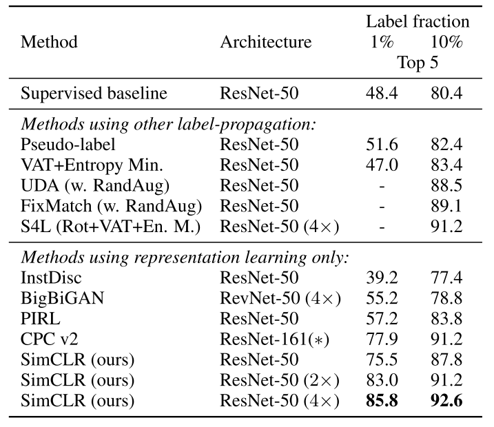] .caption[ImageNet accuracy of models trained with few labels] ] .kol-6-12[ <br><br><br> <br> <br> 1. Sample $1\\%$ or $10\\%$ of ImageNet images in a class-balanced way (i.e. $12.8 / 128$ images per class) 2. Fine-tune the whole base network on the labeled data <!-- - The supervised baseline from .citet[Zhai et al. (2019)] is strong due to intensive hyper-parameter search --> ] ] .citation[X. Zhai et al., S4L: Self-Supervised Semi-Supervised Learning, ICCV 2019 <br/> T. Chen et al., A Simple Framework for Contrastive Learning of Visual Representations, ArXiv 2020 ] ??? - Recent self-supervised methods outperform the supervised baseline --- # Efficient classification .grid[ .kol-6-12[ .center.width-100[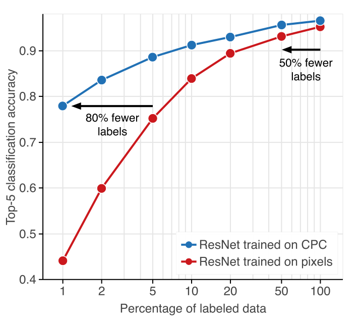] .caption[ImageNet accuracy of models trained with few labels: CPCv2 vs. supervised] ] .kol-6-12[ <br><br><br> <br> - Supervised networks do not generalize well from few labeled data - Self-supervised networks reach significantly better accuracy in the low data regime ] ] .citation[O. Henaff et al., Data-Efficient Image Recognition with Contrastive Predictive Coding, ArXiv 2019 ] --- # Transfer learning .center.width-70[] - The pre-trained model is augmented with task specific modules (e.g. decoders for semantic segmentation, RPN for object detection) and fine-tuned partially or completely - .bold[Tasks and datasets:] + Object detection: VOC07, VOC12, COCO14 + Semantic segmentation: VOC07, Cityscapes + Surface Normal Estimation: NYUv2 + Visual Navigation: Gibson .citation[ P. Goyal et al., Scaling and Benchmarking Self-Supervised Visual Representation Learning, ICCV 2019 ] --- # Transfer learning - object detection <br/> .center.width-50[] .caption[Object detection with Faster R-CNN fine-tuned on VOC $\texttt{trainval07+12}$ and evaluated on $\texttt{test07}$. <br/>Networks are pre-trained with self-supervision on ImageNet.] .citation[S. Gidaris et al., Learning Representations by Predicting Bags of Visual Words, CVPR 2020] --- class: middle # Evaluating Self-Supervised methods ## Ablation studies --- class: middle .bigger[In the last year, multiple works evaluated thoroughly self-supervised methods at scale on multiple downstream tasks and different pre-training datasets.] .bigger[We will cover only a fraction of their findings.] .citation[A. Kolesnikov et al., Revisiting Self-Supervised Visual Representation Learning, CVPR 2019 <br/> P. Goyal et al., Scaling and Benchmarking Self-Supervised Visual Representation Learning, ICCV 2019 <br/> X. Zhai et al., A Large-scale Study of Representation Learning with the Visual Task Adaptation Benchmark, ArXiv 2019 <br/> A. Newell and J. Deng, How Useful is Self-Supervised Pretraining for Visual Tasks?, CVPR 2020 <br/> B. Wallace and B. Hariharan, Extending and Analyzing Self-Supervised Learning Across Domains, ArXiv 2020] --- count: false class: middle ## Key findings - .bigger[Large impact of CNN architecture .cites[[Kolesnikov et al. (2019)]]] .hidden[ - .bigger[Increasing the size of pre-training dataset benefits higher capacity networks .cites[[Goyal et al. (2019)]]] ] .hidden[ - .bigger[Varying benefits of increasing the pretext task difficulty .cites[[Goyal et al. (2019), Chen et al. (2020)]]] ] .hidden[ - .bigger[Currently greatest benefits are in low annotated data regimes .cites[[Henaff et al. (2019); Newell and Deng (2020)]]] ] .hidden[ - .bigger[In stage 2, linear classification achieves lower performance than finetuning .cites[[Zhai et al. (2019); Newell and Deng (2020)]]] ] ??? - e.g. for _Rotation_, RevNet50 $\gg$ ResNet50 --- count: false class: middle ## Key findings - .bigger[Large impact of CNN architecture .cites[[Kolesnikov et al. (2019)]]] - .bigger[Increasing the size of pre-training dataset benefits higher capacity networks .cites[[Goyal et al. (2019)]]] .hidden[ - .bigger[Varying benefits of increasing the pretext task difficulty .cites[[Goyal et al. (2019), Chen et al. (2020)]]] ] .hidden[ - .bigger[Currently greatest benefits are in low annotated data regimes .cites[[Henaff et al. (2019); Newell and Deng (2020)]]] ] .hidden[ - .bigger[In stage 2, linear classification achieves lower performance than finetuning .cites[[Zhai et al. (2019); Newell and Deng (2020)]]] ] ??? - ResNet50 $\gt$ AlexNet - _Jigsaw_ performs better than _Colorization_. - The performance of the _Jigsaw_ model saturates (log- linearly) as we increase the data scale from 1M to 100M. --- count: false class: middle ## Key findings - .bigger[Large impact of CNN architecture .cites[[Kolesnikov et al. (2019)]]] - .bigger[Increasing the size of pre-training dataset benefits higher capacity networks .cites[[Goyal et al. (2019)]]] - .bigger[Varying benefits of increasing the pretext task difficulty .cites[[Goyal et al. (2019), Chen et al. (2020)]]] .hidden[ - .bigger[Currently greatest benefits are in low annotated data regimes .cites[[Henaff et al. (2019); Newell and Deng (2020)]]] ] .hidden[ - .bigger[In stage 2, linear classification achieves lower performance than finetuning .cites[[Zhai et al. (2019); Newell and Deng (2020)]]] ] ??? - for _Jigsaw_ we see an improvement in transfer learning performance with increased complexity - _Colorization_ appears to be less sensitive to changes in problem complexity --- count: false class: middle ## Key findings - .bigger[Large impact of CNN architecture .cites[[Kolesnikov et al. (2019)]]] - .bigger[Increasing the size of pre-training dataset benefits higher capacity networks .cites[[Goyal et al. (2019)]]] - .bigger[Varying benefits of increasing the pretext task difficulty .cites[[Goyal et al. (2019), Chen et al. (2020)]]] - .bigger[Currently greatest benefits are in low annotated data regimes .cites[[Henaff et al. (2019); Newell and Deng (2020)]]] .hidden[ - .bigger[In stage 2, linear classification achieves lower performance than finetuning .cites[[Zhai et al. (2019); Newell and Deng (2020)]]] ] --- count: false class: middle ## Key findings - .bigger[Large impact of CNN architecture .cites[[Kolesnikov et al. (2019)]]] - .bigger[Increasing the size of pre-training dataset benefits higher capacity networks .cites[[Goyal et al. (2019)]]] - .bigger[Varying benefits of increasing the pretext task difficulty .cites[[Goyal et al. (2019), Chen et al. (2020)]]] - .bigger[Currently greatest benefits are in low annotated data regimes .cites[[Henaff et al. (2019); Newell and Deng (2020)]]] - .bigger[In stage 2, linear classification achieves lower performance than finetuning .cites[[Zhai et al. (2019); Newell and Deng (2020)]]] ??? - Linear classification achieves lower performance than finetuning - Overall linear evaluation is a poor proxy for overall reduced sample complexity --- class: middle ## .center[Representation learning stress test ] .center.width-70[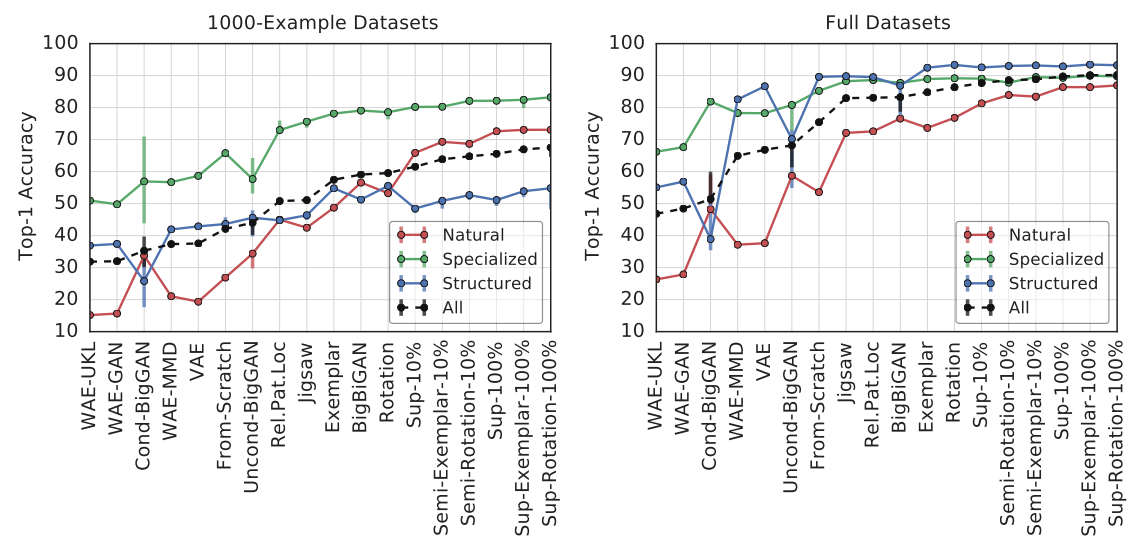] .caption[Average top-1 accuracy across the $19$ tasks in VTAB. On the x-axis the methods are ordered according to their average accuracy across all tasks.] - Self-supervised outperforms .italic[from-scratch] training. - With self-supervision, strong benefits can be obtained with fewer labels, e.g. _Sup-Rot-10%_, or all labels, e.g. _Sup-Rot-100%_, _Sup-Exemplar-100%_ .citation[X. Zhai et al., A Large-scale Study of Representation Learning with the Visual Task Adaptation Benchmark, ArXiv 2019] --- count: false class: middle ## .center[Representation learning stress test ] .center.width-70[] .caption[Average top-1 accuracy across the $19$ tasks in VTAB. On the x-axis the methods are ordered according to their average accuracy across all tasks.] - Self-supervised outperforms .italic[from-scratch] training. - .highlight[With self-supervision, strong benefits can be obtained with fewer labels, e.g. _Sup-Rot-10%_, or all labels, e.g. _Sup-Rot-100%_, _Sup-Exemplar-100%_] .citation[X. Zhai et al., A Large-scale Study of Representation Learning with the Visual Task Adaptation Benchmark, ArXiv 2019] --- class: middle, center # 5. Applications of Self-Supervision <!-- .bigg.highlight[Andrei] --> --- class: middle .bigger[Self-supervision has been successfully leveraged for several areas:] .hidden.bigger[ - Apply on downstream task with few(er) or no labels .cites[[Dwibedi et al. (2019); Wang et al. (2019); Henaff et al. (2019); Arandjelovic and Zisserman (2017)]] ] .hidden.bigger[ - Boosting performance through _an extra prediction head_ in addition to the main task: semi-supervised learning, domain generalization, etc. ] .hidden.citation[D. Dwibedi et al., Temporal Cycle-Consistency Learning, CVPR 2019 <br/> X. Wang et al., Learning Correspondence from the Cycle-Consistency of Time, CVPR 2019 <br/> O. Henaff et al., Data-Efficient Image Recognition with Contrastive Predictive Coding, ArXiv 2019 <br/> R. Arandjelovic and A. Zisserman, Look, Listen and Learn , ICCV 2017] --- count: false class: middle .bigger[Self-supervision has been successfully leveraged for several areas:] .bigger[ - Apply on downstream task with few(er) or no labels .cites[[Dwibedi et al. (2019); Wang et al. (2019); Henaff et al. (2019); Arandjelovic and Zisserman (2017)]] ] .hidden.bigger[ - Boosting performance through _an extra prediction head_ in addition to the main task: semi-supervised learning, domain generalization, etc. ] .citation[D. Dwibedi et al., Temporal Cycle-Consistency Learning, CVPR 2019 <br/> X. Wang et al., Learning Correspondence from the Cycle-Consistency of Time, CVPR 2019 <br/> O. Henaff et al., Data-Efficient Image Recognition with Contrastive Predictive Coding, ArXiv 2019 <br/> R. Arandjelovic and A. Zisserman, Look, Listen and Learn , ICCV 2017] --- count: false class: middle .bigger[Self-supervision has been successfully leveraged for several areas:] .bigger[ - Apply on downstream task with few(er) or no labels .cites[[Dwibedi et al. (2019); Wang et al. (2019); Henaff et al. (2019); Arandjelovic and Zisserman (2017)]] ] .bigger[ - Boosting performance through _an extra prediction head_ in addition to the main task: semi-supervised learning, domain generalization, etc. ] .citation[D. Dwibedi et al., Temporal Cycle-Consistency Learning, CVPR 2019 <br/> X. Wang et al., Learning Correspondence from the Cycle-Consistency of Time, CVPR 2019 <br/> O. Henaff et al., Data-Efficient Image Recognition with Contrastive Predictive Coding, ArXiv 2019 <br/> R. Arandjelovic and A. Zisserman, Look, Listen and Learn , ICCV 2017] --- count: false class: middle .inactive.bigger[Self-supervision has been successfully leveraged for several areas:] .inactive.bigger[ - Apply on downstream task with few(er) or no labels .cites[.inactive[[Dwibedi et al. (2019); Wang et al. (2019); Henaff et al. (2019); Arandjelovic and Zisserman (2017)]]] ] .bigger[ - Boosting performance through _an extra prediction head_ in addition to the main task: semi-supervised learning, domain generalization, etc. ] .citation[D. Dwibedi et al., Temporal Cycle-Consistency Learning, CVPR 2019 <br/> X. Wang et al., Learning Correspondence from the Cycle-Consistency of Time, CVPR 2019 <br/> O. Henaff et al., Data-Efficient Image Recognition with Contrastive Predictive Coding, ArXiv 2019 <br/> R. Arandjelovic and A. Zisserman, Look, Listen and Learn , ICCV 2017] --- class: middle ## .center[Bridging few-shot and self-supervised learning] .center.width-75[] - Both paradigms aim to learn from few or no labeled images and consist of two stages - .bold[Self-supervision as auxiliary objective] at 1st learning stage of few-shot model: - More diverse features and better ability to adapt to novel classes with few data - Explored self-supervised methods: _Rotation_ and _Relative Patch Location_ .citation[S. Gidaris et al., Boosting Few-Shot Learning with Self-Supervision, ICCV 2019; J.C. Su et al., When Does Self-supervision Improve Few-shot Learning?, ArXiv 2019] --- class: middle ## .center[Towards better robustness and uncertainty] .grid[ .kol-4-12[ <br/><br/><br/> .center.width-80[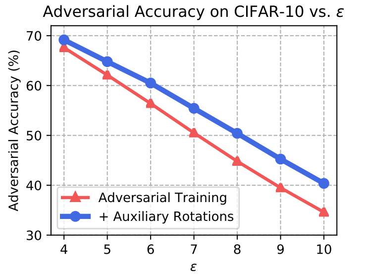] .caption[Accuracy under adversarial attacks of varying strenghts $\varepsilon$] ] .kol-8-12[ .center.width-85[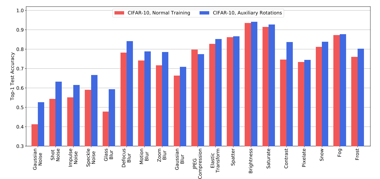] .caption[ Accuracy of usual training vs training with auxiliary rotation self-supervision on the 19 CIFAR-10-C corruptions.] ] ] .hidden[ .center.width-25[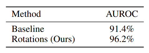] .caption[Out-of-Distribution detection performance] ] .citation[D. Hendrycks et al., Using Self-Supervised Learning Can Improve Model Robustness and Uncertainty, NIPS 2019; F. Ahmed & A. Courville, Detecting semantic anomalies, AAAI 2020] --- count: false class: middle ## .center[Towards better robustness and uncertainty] .grid[ .kol-4-12[ <br/><br/><br/> .center.width-80[] .caption[Accuracy under adversarial attacks of varying strenghts $\varepsilon$] ] .kol-8-12[ .center.width-85[] .caption[ Accuracy of usual training vs training with auxiliary rotation self-supervision on the 19 CIFAR-10-C corruptions.] ] ] .center.width-25[] .caption[Out-of-Distribution detection performance] .citation[D. Hendrycks et al., Using Self-Supervised Learning Can Improve Model Robustness and Uncertainty, NIPS 2019; F. Ahmed & A. Courville, Detecting semantic anomalies, AAAI 2020] --- class: middle ## .center[Domain generalization and adaptation] .center.width-90[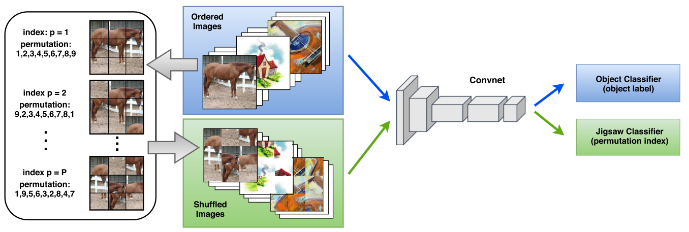] - Recognizing objects across visual domains requires high generalization abilities. - Signals from pretext tasks allow to capture natural invariances and regularities in data. .citation[F.M. Carlucci et al., Domain Generalization by Solving Jigsaw Puzzles, CVPR 2019] ??? - Signals from self-supervised pretext tasks allow to capture natural invariances and regularities in data that could mitigate large style gaps. --- class: middle .center.width-60[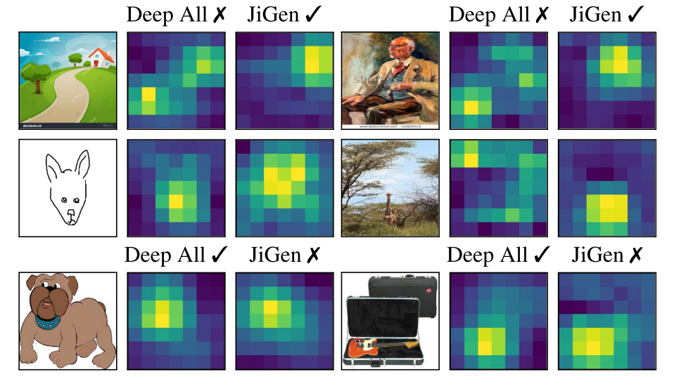] .caption[CAM activation maps: yellow corresponds to high values, while dark blue corresponds to low values.] The self-supervised pretext task enables localization of the most informative part of the image, useful for object class prediction regardless of the visual domain. .citation[F.M. Carlucci et al., Domain Generalization by Solving Jigsaw Puzzles, CVPR 2019] --- class: middle ## .center[Rotation for better GAN Discriminators] .grid[ .kol-6-12[ .center.width-100[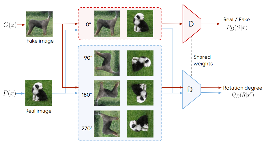] .caption[Discriminator with rotation-based self-supervision. ] ] .kol-6-12[ <br/> <br/> - Add self-supervised auxiliary task to .italic[Discriminator] - Encourage the .italic[Discriminator] to learn meaningful feature representations which are not forgotten during training <!-- - Self-supervised unconditional GAN reaches similar performance to state-of-the-art conditional counterparts --> ] ] .citation[T. Chen et al., Self-Supervised GANs via Auxiliary Rotation Loss, CVPR 2019] ??? - Both the fake and real images are rotated by $0\degree$, $90\degree$, $180\degree$, and $270\degree$ degrees. The colored arrows indicate that only the upright images are considered for true vs. fake classification loss task. For the rotation loss, all images are classified by the discriminator according to their rotation degree. - Self-supervised unconditional GAN reaches similar performance to state-of-the-art conditional counterparts --- class: middle, center # 6. Open challenges <!-- .bigg.highlight[Andrei] --> --- class: middle .bigger[Although they achieve outstanding performance, contrastive methods require long training and complex setups, e.g. TPUs, large mini-batches.] .hidden.bigger[Recent works have showed that reconstruction methods can achieve competitive performance by reconstructing features instead of inputs.] .hidden.Q[Can we improve or go beyond contrastive learning?] .hidden.citation[S. Gidaris et al., Learning Representations by Predicting Bags of Visual Words, CVPR 2020 <br/> J. B. Grill et al., Bootstrap Your Own Latent: A New Approach to Self-Supervised Learning, ArXiv 2020 ] --- count: false class: middle .bigger[Although they achieve outstanding performance, contrastive methods require long training and complex setups, e.g. TPUs, large mini-batches.] .bigger[Recent works have showed that reconstruction methods can achieve competitive performance by reconstructing features instead of inputs.] .hidden.Q[Can we improve or go beyond contrastive learning?] .citation[S. Gidaris et al., Learning Representations by Predicting Bags of Visual Words, CVPR 2020 <br/> J. B. Grill et al., Bootstrap Your Own Latent: A New Approach to Self-Supervised Learning, ArXiv 2020 ] --- count: false class: middle .bigger[Although they achieve outstanding performance, contrastive methods require long training and complex setups, e.g. TPUs, large mini-batches.] .bigger[Recent works have showed that reconstruction methods can achieve competitive performance by reconstructing features instead of inputs.] .center.Q[Can we improve or go beyond contrastive learning?] .citation[S. Gidaris et al., Learning Representations by Predicting Bags of Visual Words, CVPR 2020 <br/> J. B. Grill et al., Bootstrap Your Own Latent: A New Approach to Self-Supervised Learning, ArXiv 2020 ] --- class: middle .bigger[.citet[Asano et al. (2020)] show that **as little as a single image is sufficient**, when combined with self-supervision and data augmentation, to learn the first few layers of standard deep networks as well as using millions of images and full supervision.] .citation[Y.M. Asano, A critical analysis of self-supervision, or what we can learn from a single image, ICLR 2020] --- class: middle .grid[ .kol-6-12[ .center[1 - Take a high-resolution image] <br/> .center.width-80[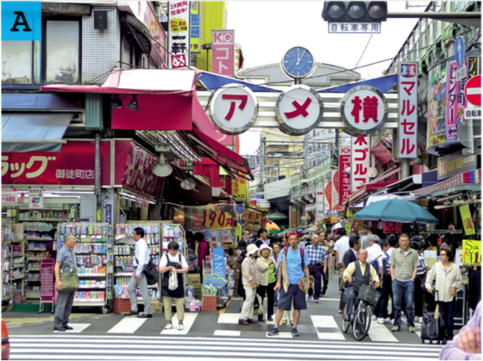] ] .hidden[ .kol-6-12[ .center[2 - Generate 1M images of crops and augmentations] <br/> .center.width-80[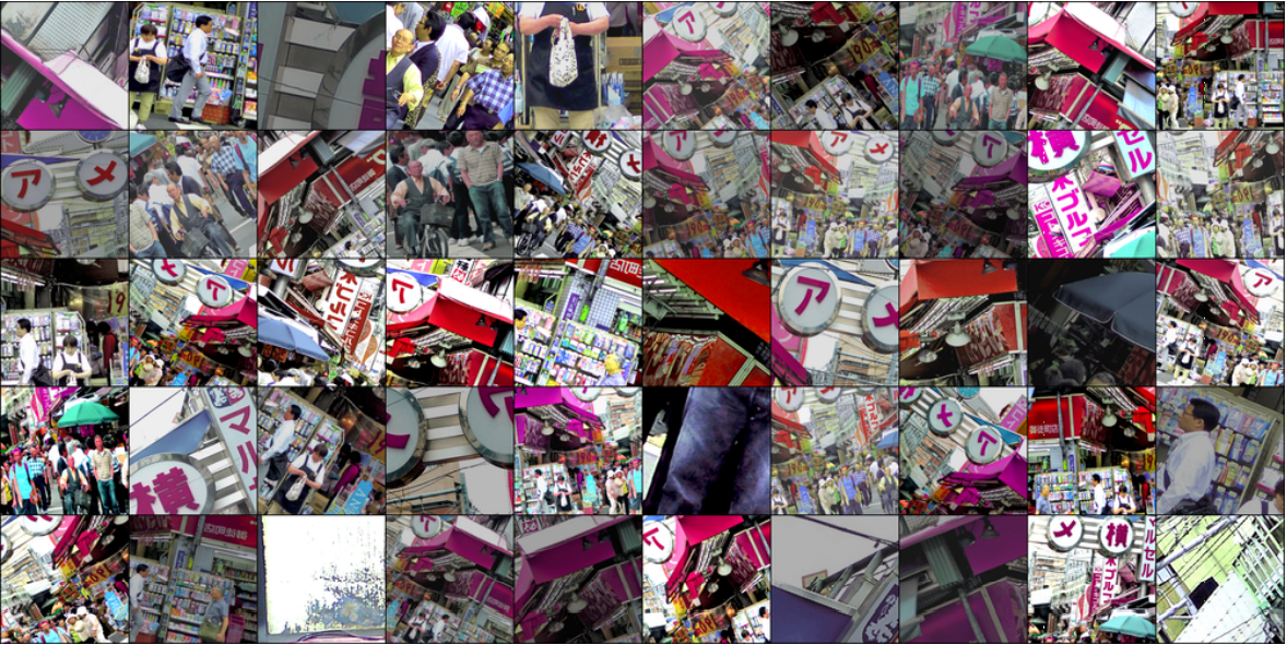] ] ] ] .hidden[.Q[How to better leverage data for extracting more sophisticated information for learning representations?]] .citation[Y.M. Asano, A critical analysis of self-supervision, or what we can learn from a single image, ICLR 2020] --- count: false class: middle .grid[ .kol-6-12[ .center[1 - Take a high-resolution image] <br/> .center.width-80[] ] .kol-6-12[ .center[2 - Generate 1M images of crops and augmentations] <br/> .center.width-80[] ] ] .hidden[.Q[How to better leverage data for extracting more sophisticated information for learning representations?]] .citation[Y.M. Asano, A critical analysis of self-supervision, or what we can learn from a single image, ICLR 2020] --- count: false class: middle .grid[ .kol-6-12[ .center[1 - Take a high-resolution image] <br/> .center.width-80[] ] .kol-6-12[ .center[2 - Generate 1M images of crops and augmentations] <br/> .center.width-80[] ] ] .center.Q[How to better leverage data for extracting more sophisticated information for learning representations?] .citation[Y.M. Asano, A critical analysis of self-supervision, or what we can learn from a single image, ICLR 2020] --- class: middle .grid[ .kol-7-12[ .center.width-100[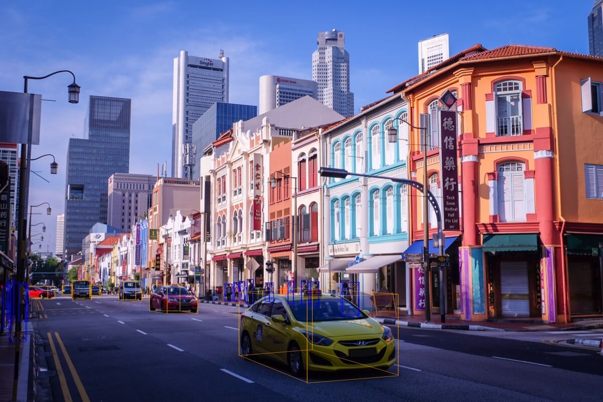] ] .kol-5-12[ <br/><br/> - With few exceptions, e.g. MonoDepth, most self-supervised methods deal with ImageNet-like data with one dominant object per image. - In the case of autonomous driving data with HD images and large complex scenes, these strategies are cumbersome to apply. ] ] .citation[H. Caesar et al., nuScenes: A multimodal dataset for autonomous driving, CVPR 2020 ] --- class: middle .center.width-100[] - Instead, in medical imaging, frequently there is little structure to exploit from images. .hidden.center.Q[How to go beyond single-object images?] .citation[E. Bejnordi et al., Diagnostic Assessment of Deep Learning Algorithms for Detection of Lymph Node Metastases in Women With Breast Cancer, JAMA 2017] --- count: false class: middle .center.width-100[] - Instead, in medical imaging, frequently there is little structure to exploit from images. .center.Q[How to go beyond single-object images?] .citation[E. Bejnordi et al., Diagnostic Assessment of Deep Learning Algorithms for Detection of Lymph Node Metastases in Women With Breast Cancer, JAMA 2017] --- class: middle # Open challenges ## Beyond contrastive learning ## Beyond learning simple image statistics ## Beyond single object images --- class: middle .big.italic.purple[".bold[Unsupervised learning:] Think hard about the model, use whatever data fits.] .big.italic.purple[.bold[Self-supervised learning:] Think hard about the data, use whatever model fits."] .bold.bigger.pull-right[Misha Denil] <br/> <br/> .center.width-30[] --- layout: false class: end-slide, center count: false The end. --- layout: true .center.footer[Andrei BURSUC and Relja ARANDJELOVIĆ | Self-Supervised Learning] --- count: false class: middle ## .center[Typical data augmentation composition (pytorch) for self-supervised learning ] <br/> .grid[ .kol-3-12[ ] .kol-6-12[ ``` from torchvision import transforms ... augmentation = [ transforms.RandomResizedCrop(224, scale=(0.2, 1.)), transforms.RandomApply([ transforms.ColorJitter(0.8, 0.8, 0.8, 0.2)], p=0.8), transforms.RandomGrayscale(p=0.2), transforms.RandomApply([GaussianBlur([0.1, 2.0])], p=0.5), transforms.RandomHorizontalFlip(), transforms.ToTensor(), transforms.Normalize(mean=[0.485, 0.456, 0.406], std=[0.229, 0.224, 0.225]) ] ``` ] .kol-3-12[ ] ] .citation[T. Chen et al., A Simple Framework for Contrastive Learning of Visual Representations, ArXiv 2020 <br/> K. He et al., Improved Baselines with Momentum Contrastive Learning, ArXiv 2020] --- count: false class: middle # Practical considerations ## Feature normalization --- count: false # Feature Normalization - the $\text{softmax}$ function generalizes the sigmoid function and yields a vector of $k$ values in $[0, 1]$ by exponentiating and then normalizing $$\text{softmax}(a)= \frac{1}{\sum\_j \exp(a\_j)} [\exp(a\_1), \dots, \exp(a\_k)]$$ - the $\text{softmax}$ distribution can be made arbitrarily sharp by simply scaling all the features .center.width-100[] .caption[$\text{softmax}$ output for different logit scales] --- count:false # Feature Normalization - the $\text{softmax}$ function generalizes the sigmoid function and yields a vector of $k$ values in $[0, 1]$ by exponentiating and then normalizing $$\text{softmax}(a)= \frac{1}{\sum\_j \exp(a\_j)} [\exp(a\_1), \dots, \exp(a\_k)]$$ - the $\text{softmax}$ distribution can be made arbitrarily sharp by simply scaling all the features .center.width-100[] .caption[$\text{softmax}$ output for different logit scales] --- count:false # Feature Normalization - the $\text{softmax}$ function generalizes the sigmoid function and yields a vector of $k$ values in $[0, 1]$ by exponentiating and then normalizing $$\text{softmax}(a)= \frac{1}{\sum\_j \exp(a\_j)} [\exp(a\_1), \dots, \exp(a\_k)]$$ - the $\text{softmax}$ distribution can be made arbitrarily sharp by simply scaling all the features .center.width-100[] .caption[$\text{softmax}$ output for different logit scales] --- count:false # Feature Normalization - the $\text{softmax}$ function generalizes the sigmoid function and yields a vector of $k$ values in $[0, 1]$ by exponentiating and then normalizing $$\text{softmax}(a)= \frac{1}{\sum\_j \exp(a\_j)} [\exp(a\_1), \dots, \exp(a\_k)]$$ - the $\text{softmax}$ distribution can be made arbitrarily sharp by simply scaling all the features .center.width-100[] .caption[$\text{softmax}$ output for different logit scales] --- count:false # Feature Normalization - the $\text{softmax}$ function generalizes the sigmoid function and yields a vector of $k$ values in $[0, 1]$ by exponentiating and then normalizing $$\text{softmax}(a)= \frac{1}{\sum\_j \exp(a\_j)} [\exp(a\_1), \dots, \exp(a\_k)]$$ - the $\text{softmax}$ distribution can be made arbitrarily sharp by simply scaling all the features .center.width-100[] .caption[$\text{softmax}$ output for different logit scales] --- count:false # Feature Normalization - the $\text{softmax}$ function generalizes the sigmoid function and yields a vector of $k$ values in $[0, 1]$ by exponentiating and then normalizing $$\text{softmax}(a)= \frac{1}{\sum\_j \exp(a\_j)} [\exp(a\_1), \dots, \exp(a\_k)]$$ - the $\text{softmax}$ distribution can be made arbitrarily sharp by simply scaling all the features .center.width-100[] .caption[$\text{softmax}$ output for different logit scales] --- count:false # Feature Normalization - the $\text{softmax}$ function generalizes the sigmoid function and yields a vector of $k$ values in $[0, 1]$ by exponentiating and then normalizing $$\text{softmax}(a)= \frac{1}{\sum\_j \exp(a\_j)} [\exp(a\_1), \dots, \exp(a\_k)]$$ - the $\text{softmax}$ distribution can be made arbitrarily sharp by simply scaling all the features .center.width-100[] .caption[$\text{softmax}$ output for different logit scales] --- count:false # Feature Normalization - the $\text{softmax}$ function generalizes the sigmoid function and yields a vector of $k$ values in $[0, 1]$ by exponentiating and then normalizing $$\text{softmax}(a)= \frac{1}{\sum\_j \exp(a\_j)} [\exp(a\_1), \dots, \exp(a\_k)]$$ - the $\text{softmax}$ distribution can be made arbitrarily sharp by simply scaling all the features .center.width-100[] .caption[$\text{softmax}$ output for different logit scales] --- count: false class: middle .bigger[$\ell\_{2}$-normalization is frequently used for normalizing features for the contrastive loss.] .bigger[Without $\ell\_{2}$-normalization, accuracy on the pretext task is usually better, $+2-5\\%$, but lower in the downstream task (even on the same dataset, e.g. ImageNet), $-7\\%$] .citation[T. Chen et al., A Simple Framework for Contrastive Learning of Visual Representations, ArXiv 2020 ] --- count: false # Temperature scaling - The temperature parameter $\tau$ controls the concentration level of the $\text{softmax}$ distribution $$ \text{softmax}(a/\tau):= \frac{1}{\sum\_j \exp(a\_j/\tau)} [\exp(a\_1/\tau), \dots, \exp(a\_k/\tau)]$$ - it mitigates the peaky predictions from $\text{softmax}$ by increasing its entropy $$\tau=1$$ .center.width-90[] .caption[Impact of temperature scaling on non-normalized logits] .citation[G. Hinton et al., Distilling the knowledged in a neural network, ArXiv 2015] --- count: false # Temperature scaling - The temperature parameter $\tau$ controls the concentration level of the $\text{softmax}$ distribution $$ \text{softmax}(a/\tau):= \frac{1}{\sum\_j \exp(a\_j/\tau)} [\exp(a\_1/\tau), \dots, \exp(a\_k/\tau)]$$ - it mitigates the peaky predictions from $\text{softmax}$ by increasing its entropy $$\tau=2$$ .center.width-90[] .caption[Impact of temperature scaling on non-normalized logits] .citation[G. Hinton et al., Distilling the knowledged in a neural network, ArXiv 2015] --- count: false # Temperature scaling - The temperature parameter $\tau$ controls the concentration level of the $\text{softmax}$ distribution $$ \text{softmax}(a/\tau):= \frac{1}{\sum\_j \exp(a\_j/\tau)} [\exp(a\_1/\tau), \dots, \exp(a\_k/\tau)]$$ - it mitigates the peaky predictions from $\text{softmax}$ by increasing its entropy $$\tau=5$$ .center.width-90[] .caption[Impact of temperature scaling on non-normalized logits] .citation[G. Hinton et al., Distilling the knowledged in a neural network, ArXiv 2015] --- count: false # Temperature scaling - The temperature parameter $\tau$ controls the concentration level of the $\text{softmax}$ distribution $$ \text{softmax}(a/\tau):= \frac{1}{\sum\_j \exp(a\_j/\tau)} [\exp(a\_1/\tau), \dots, \exp(a\_k/\tau)]$$ - it mitigates the peaky predictions from $\text{softmax}$ by increasing its entropy $$\tau=10$$ .center.width-90[] .caption[Impact of temperature scaling on non-normalized logits] .citation[G. Hinton et al., Distilling the knowledged in a neural network, ArXiv 2015] --- count: false # Temperature scaling - The temperature parameter $\tau$ controls the concentration level of the $\text{softmax}$ distribution $$ \text{softmax}(a/\tau):= \frac{1}{\sum\_j \exp(a\_j/\tau)} [\exp(a\_1/\tau), \dots, \exp(a\_k/\tau)]$$ - it mitigates the peaky predictions from $\text{softmax}$ by increasing its entropy $$\tau=20$$ .center.width-90[] .caption[Impact of temperature scaling on non-normalized logits] .citation[G. Hinton et al., Distilling the knowledged in a neural network, ArXiv 2015] --- count: false # Temperature scaling - The temperature parameter $\tau$ controls the concentration level of the $\text{softmax}$ distribution $$ \text{softmax}(a/\tau):= \frac{1}{\sum\_j \exp(a\_j/\tau)} [\exp(a\_1/\tau), \dots, \exp(a\_k/\tau)]$$ - it mitigates the peaky predictions from $\text{softmax}$ by increasing its entropy $$\tau=50$$ .center.width-90[] .caption[Impact of temperature scaling on non-normalized logits] .citation[G. Hinton et al., Distilling the knowledged in a neural network, ArXiv 2015] --- count: false # Temperature scaling - The temperature parameter $\tau$ controls the concentration level of the $\text{softmax}$ distribution $$ \text{softmax}(a/\tau):= \frac{1}{\sum\_j \exp(a\_j/\tau)} [\exp(a\_1/\tau), \dots, \exp(a\_k/\tau)]$$ - it mitigates the peaky predictions from $\text{softmax}$ by increasing its entropy $$\tau=100$$ .center.width-90[] .caption[Impact of temperature scaling on non-normalized logits] .citation[G. Hinton et al., Distilling the knowledged in a neural network, ArXiv 2015] --- count: false # Temperature scaling - The temperature parameter $\tau$ controls the concentration level of the $\text{softmax}$ distribution $$ \text{softmax}(a/\tau):= \frac{1}{\sum\_j \exp(a\_j/\tau)} [\exp(a\_1/\tau), \dots, \exp(a\_k/\tau)]$$ - it mitigates the peaky predictions from $\text{softmax}$ by increasing its entropy $$\tau=400$$ .center.width-90[] .caption[Impact of temperature scaling on non-normalized logits] .citation[G. Hinton et al., Distilling the knowledged in a neural network, ArXiv 2015] --- count: false class: middle .bigger[ The optimum value of $\tau$ depends whether logits are normalized or not or if they are followed by a non-linear projection Some .italic[rules-of-thumb] *(when extensive hyper-parameter search is not an option)*: - no $\ell\_2$-normalization: $\tau \in [10, 100]$.cites[[Chen et al. (2020)]] - $\ell\_2$-normalized vectors: $\tau \in [0.07, 0.1]$ .cites[[Wu et al. (2018), He et al. (2020), Chen et al. (2020)]] - $\ell\_2$-normalized vectors + non-linear projection: $\tau = 0.2$ .cites[[He et al. (2020)]] ] .citation[Z. Wu et al., Unsupervised Feature Learning via Non-Parametric Instance Discrimination, CVPR 2018 <br/> K. He et al., Momentum Contrast for Unsupervised Visual Representation Learning, CVPR 2020 <br/> T. Chen et al., A Simple Framework for Contrastive Learning of Visual Representations, ArXiv 2020 <br/> K. He et al., Improved Baselines with Momentum Contrastive Learning, ArXiv 2020 ] --- count: false class: middle .center.width-55[] .caption[Linear evaluation for models trained with different choices of <br/> $\ell\_2$-normalization and temperature $\tau$ for contrastive loss with 4096 samples.] .citation[T. Chen et al., A Simple Framework for Contrastive Learning of Visual Representations, ArXiv 2020 ] --- count: false class: middle # Practical considerations ## Hyperparameters for pretext and downstream tasks --- count: false class: middle .grid[ .kol-6-12[ .center.bold[*Stage 1:* Train network on pretext task (without human labels) ] .center.width-100[] .center.bold[*Stage 2:* Train classifier on learned features for new task with fewer labels] .center.width-100[] ] .kol-6-12[ .hidden[ <br/> - For the _Linear Classification Protocol_, hyperparameter tuning was limited in order to emphasize the utility of the learned features. - .citet[Tian et al. (2019)] and .citet[He et al. (2020)] observed that feature distributions from pretext tasks can be substantially different from supervised ones - This leads to different hyperparamater values: __weight decay = $0$__, __initial learning rate = $30$__ ] ] ] .hidden[ .citation[Y. Tian et al.Contrastive Multiview Coding, ArXiv 2019 <br/> K. He et al., Momentum Contrast for Unsupervised Visual Representation Learning, CVPR 2020 ] ] --- count: false class: middle .grid[ .kol-6-12[ .center.bold[*Stage 1:* Train network on pretext task (without human labels) ] .center.width-100[] .center.bold[*Stage 2:* Train classifier on learned features for new task with fewer labels] .center.width-100[] ] .kol-6-12[ .hidden[ <br/> - For the _Linear Classification Protocol_, hyperparameter tuning was limited in order to emphasize the utility of the learned features. - .citet[Tian et al. (2019)] and .citet[He et al. (2020)] observed that feature distributions from pretext tasks can be substantially different from supervised ones - This leads to different hyperparamater values: __weight decay = $0$__, __initial learning rate = $30$__ ] ] ] .hidden[ .citation[Y. Tian et al.Contrastive Multiview Coding, ArXiv 2019 <br/> K. He et al., Momentum Contrast for Unsupervised Visual Representation Learning, CVPR 2020 ] ] --- count: false class: middle .grid[ .kol-6-12[ .center.bold[*Stage 1:* Train network on pretext task (without human labels) ] .center.width-100[] .center.bold[*Stage 2:* Train classifier on learned features for new task with fewer labels] .center.width-100[] ] .kol-6-12[ <br/> - For the _Linear Classification Protocol_, hyperparameter tuning was limited in order to emphasize the utility of the learned features. - .citet[Tian et al. (2019)] and .citet[He et al. (2020)] observed that feature distributions from pretext tasks can be substantially different from supervised ones - This leads to different hyperparamater values: __weight decay = $0$__, __initial learning rate = $30$__ ] ] .citation[Y. Tian et al.Contrastive Multiview Coding, ArXiv 2019 <br/> K. He et al., Momentum Contrast for Unsupervised Visual Representation Learning, CVPR 2020 ] --- count: false class: middle .grid[ .kol-6-12[ .center.bold[*Stage 1:* Train network on pretext task (without human labels) ] .center.width-100[] .center.bold[*Stage 2:* Train classifier on learned features for new task with fewer labels] .center.width-100[] ] .kol-6-12[ <br/><br/><br/> - Similarly for fine-tuning, we can train BatchNorm layers instead of converting them into frozen affine layers. - This leads to performance boosts on different tasks: object detection, semantic segmentation. ] ] .citation[K. He et al., Momentum Contrast for Unsupervised Visual Representation Learning, CVPR 2020 ] --- count: false class:middle ## .center[Impact of the architecture] .grid[ .kol-6-12[ .center.width-100[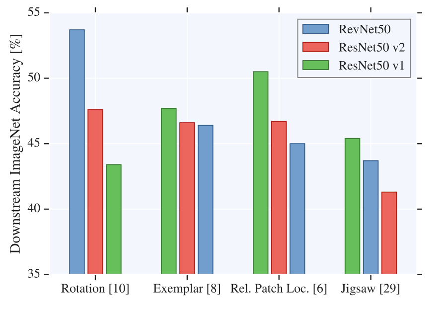] ] .kol-6-12[ <br/><br/><br/><br/><br/> Quality of visual representations learned by various self-supervised learning techniques depends significantly on the CNN architecture used for the pretext task. ] ] .citation[A. Kolesnikov et al., Revisiting Self-Supervised Visual Representation Learning, CVPR 2019] --- count: false class:middle ## .center[Using more data for pre-training] .grid[ .kol-6-12[ .center.width-100[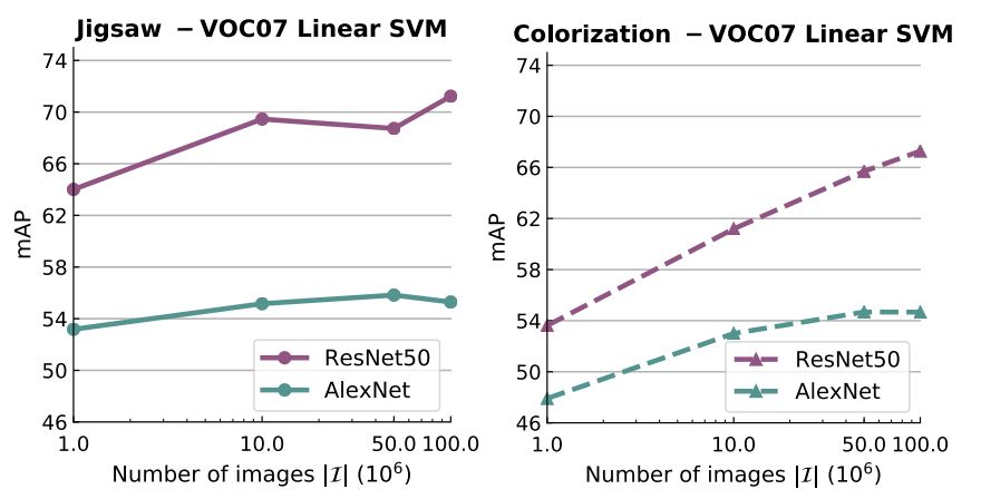] .caption[Transfer learning performance of self-supervised methods on the VOC07 dataset for AlexNet and ResNet-50 when varying the size of the pre-training dataset (ImageNet + YFCC-100M) ] ] .kol-6-12[ - Increasing the size of pre-training data improves the transfer learning performance for both the _Jigsaw_ and _Colorization_ methods on ResNet-50 and AlexNet. - _Jigsaw_ performs better than _Colorization_. - The performance of the _Jigsaw_ model saturates (log- linearly) as we increase the data scale from 1M to 100M. - performance gap between AlexNet and ResNet-50 keeps increasing, suggesting that higher capacity models are needed to take full advantage of the larger pre-training datasets. ] ] .citation[ P. Goyal et al., Scaling and Benchmarking Self-Supervised Visual Representation Learning, ICCV 2019] --- count: false class:middle ## .center[Increasing problem complexity] .grid[ .kol-6-12[ .center.width-100[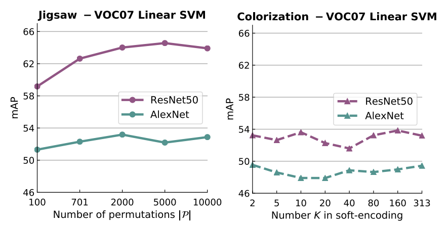] .caption[Transfer learning performance of _Jigsaw_ and _Colorization_ on VOC07 dataset for AlexNet and ResNet-50 when varying pretext problem complexity. ] ] .kol-6-12[ <br/> <br/> - for _Jigsaw_ we see an improvement in transfer learning performance with increased complexity - _Colorization_ appears to be less sensitive to changes in problem complexity ] ] .citation[ P. Goyal et al., Scaling and Benchmarking Self-Supervised Visual Representation Learning, ICCV 2019] --- count: false class: middle .bigger[.citet[Newell and Deng (2020)] show that the __greatest benefits of pretraining are currently in low data regimes__, and utility approaches zero before performance plateaus on the task from additional labels.] .bigger[This finding underpins the usefulness of self-supervised learning when limited annotation data is available.] .citation[A. Newell and J. Deng, How Useful is Self-Supervised Pretraining for Visual Tasks?, CVPR 2020] --- count: false class: middle ## .center[Changing domains for both pre-training and downstream datasets] .grid[ .kol-6-12[ .center.width-100[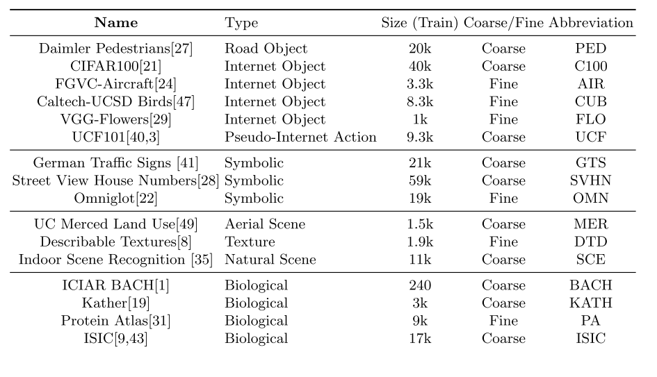] .caption[List of 16 datasets evaluated in .cites[[Wallace and Hariharan (2020)]]. They are into 4 categories: .bold[Internet], .bold[Symbolic], .bold[Scenes & Textures], and .bold[Biological].] ] .kol-6-12[ <br/> - Self-supervised techniques: _Rotation_, _Jigsaw_, _NPID_, _Autoencoders_ - _Rotation_ is the most semantically meaningful task - Much of the performance of _Jigsaw_ and _NPID_ comes from the nature of their induced distribution rather than semantic understanding - There are still several areas, e.g. fine-grained classification, where all tasks underperform. ] ] .citation[ B. Wallace and B. Hariharan, Extending and Analyzing Self-Supervised Learning Across Domains, ArXiv 2020] --- count: false class: middle <!-- ## .center[Comparison to other representation learning methods. ] --> ## .center[Representation learning stress test ] .center.width-60[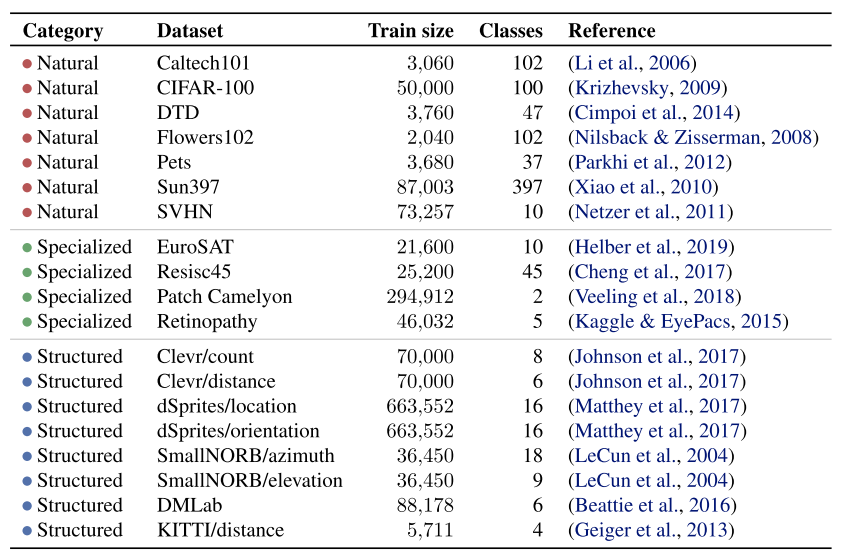] .caption[The 19 datasets of the Visual Task Adaptation Benchmark (VTAB). <br/> They are grouped into three sets: .bold[Natural], .bold[Specialized], .bold[Structured]. ] .citation[X. Zhai et al., A Large-scale Study of Representation Learning with the Visual Task Adaptation Benchmark, ArXiv 2019] --- count: false class: middle <!-- ## .center[Comparison to other representation learning methods. ] --> ## .center[Representation learning stress test ] .center.width-60[] .caption[The 19 datasets of the Visual Task Adaptation Benchmark (VTAB). <br/> They are grouped into three sets: .bold[Natural], .bold[Specialized], .bold[Structured]. ] .citation[X. Zhai et al., A Large-scale Study of Representation Learning with the Visual Task Adaptation Benchmark, ArXiv 2019] --- count: false class: middle ## .center[Representation learning stress test ] .center.width-70[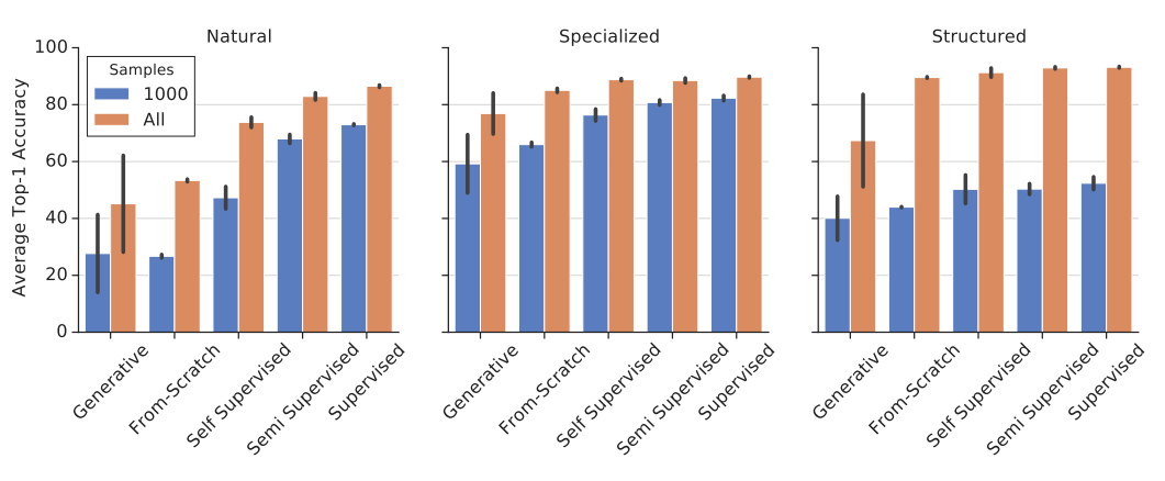] .caption[Aggregated performance of each method group: .bold[generative] (VAE, WAE, BigGAN, BigBiGAN), .bold[training from-scratch], .bold[self-supervised], .bold[semi-supervised] (*Rotation*, *Exemplar*, *Relative Patch Location*, *Jigsaw*) (using $10\\%$ ImageNet labels), .bold[supervised] (using $100\\%$ ImageNet labels).<br/> .bold[All]: using all labeled images from downstream task; .bold[1000]: using 100 annotated images] - Self-supervised out-performs .italic[from-scratch] training. - Interestingly, on .bold[Structured] tasks self-supervised methods perform slightly better than supervised ones. .citation[X. Zhai et al., A Large-scale Study of Representation Learning with the Visual Task Adaptation Benchmark, ArXiv 2019] ??? - This indicates supervised ImageNet models are invariant to useful features required for structured understanding, but self-supervised methods can capture these to some degree --- count: false class: middle ## .center[Linear classification vs. fine-tuning] .grid[ .kol-6-12[ .center.width-100[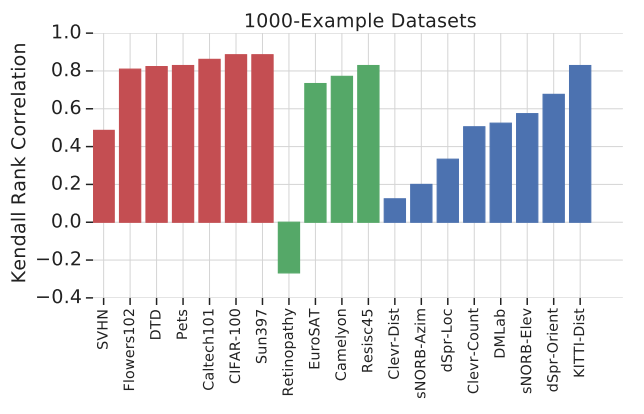] .caption[Kendall’s correlation between fine-tuning and linear evaluation on each dataset.] ] .kol-6-12[ <br/><br/><br/> - Linear classification significantly lowers performance - Overall linear evaluation is a poor proxy for overall reduced sample complexity - A similar result was found by .citet[Newell and Deng (2020)] ] ] .citation[X. Zhai et al., A Large-scale Study of Representation Learning with the Visual Task Adaptation Benchmark, ArXiv 2019 <br/> A. Newell and J. Deng, How Useful is Self-Supervised Pretraining for Visual Tasks?, CVPR 2020] --- class: middle .grid[ .kol-6-12[ .center.width-100[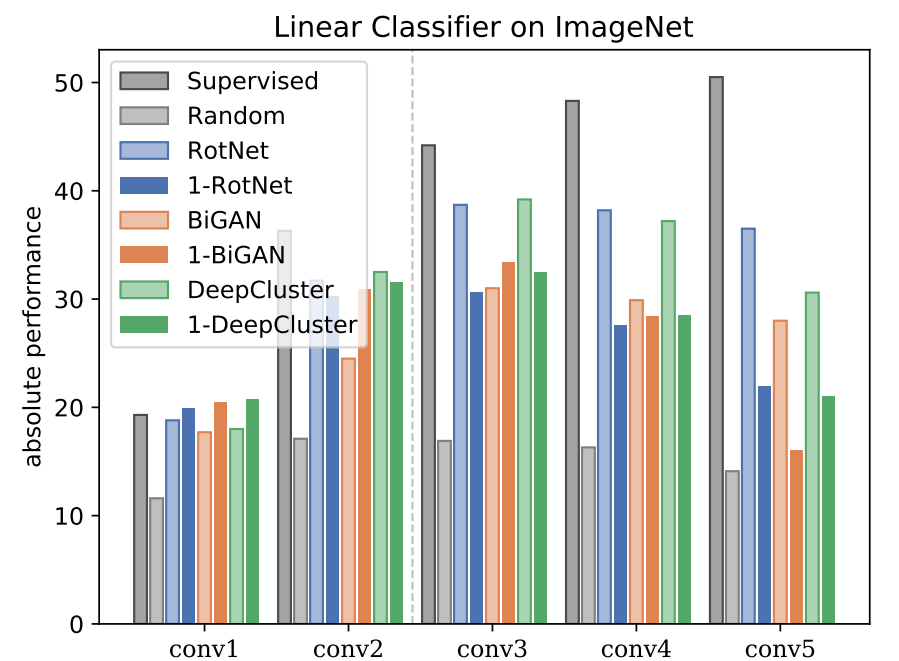] .caption[Accuracies of linear classifiers trained on the representations from intermediate layers of supervised and self-supervised network ] ] .kol-6-12[ <br/><br/><br/> - With sufficient data augmentation, one image allows self-supervision to learn good and generalizable features - At deeper layers there is a gap with supervised methods, that is mitigated to some extent by large datasets for self-supervised methods ] ] .hidden[.Q[How to better leverage data for extracting more sophisticated information for learning representations?]] .citation[Y.M. Asano, A critical analysis of self-supervision, or what we can learn from a single image, ICLR 2020]