layout: true <div class="header-logo"><img src="images/eccv-logo.svg" /></div> .center.footer[Andrei BURSUC | A Bayesian Odyssey in Uncertainty: Introduction ] --- class: center, middle ## ECCV 2024 Tutorial # A Bayesian Odyssey in Uncertainty: <br> from Theoretical Foundations to Real-World Applications <br> .grid[ .kol-4-12[ .bold[Gianni Franchi] ] .kol-4-12[ .bold[Adrien Lafage] ] .kol-4-12[ .bold[Olivier Laurent] ] ] .grid[ .kol-4-12[ .bold[Alexander Immer] ] .kol-4-12[ .bold[Pavel Izmailov] ] .kol-4-12[ .bold[Andrei Bursuc] ] ] .foot[https://uqtutorial.github.io/] --- count: false class: middle .center.width-75[] --- class: center, middle ## ECCV 2024 Tutorial <!-- ## A Bayesian Odyssey in Uncertainty: <br> from Theoretical Foundations to Real-World Applications --> # Introduction <br/> .center.big.bold[Andrei Bursuc] .center[<img src="images/logo_valeoai.png" style="width: 200px;" />] .foot[https://uqtutorial.github.io/] --- class: middle ## A decade of mad progress .center.width-80[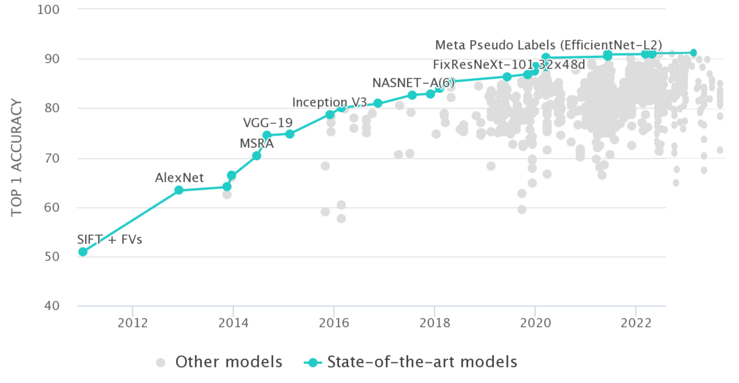] .center.bigger[ImageNet-1k image **classification**] --- class: middle ## A decade of mad progress .center.width-75[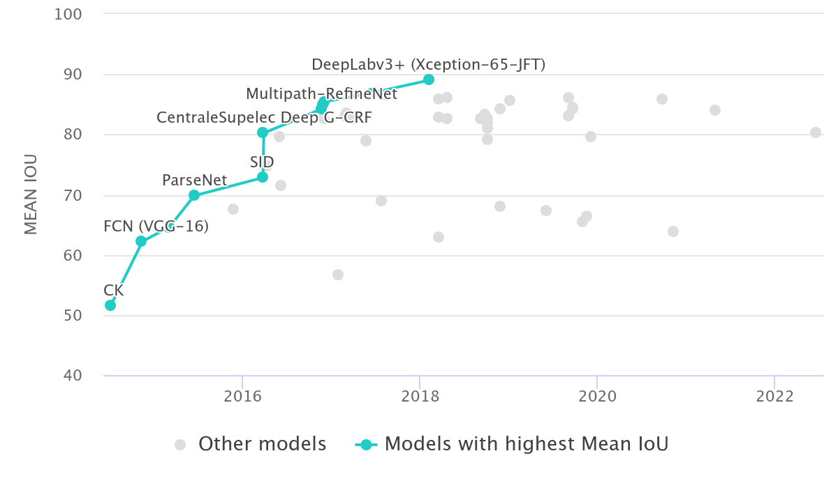] .center.bigger[Pascal-VOC **semantic segmentation**] --- class: middle ## A decade of mad progress .center.width-75[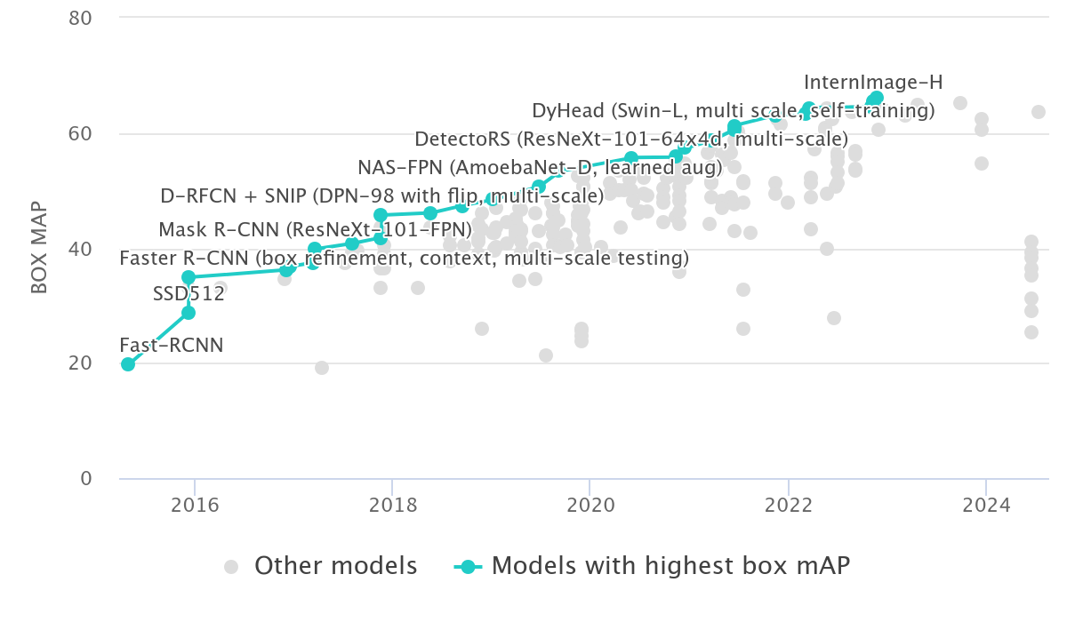] .center.bigger[MC-COCO **object detection**] --- class: middle, center .big[There are plenty of real-world cases where such models would be useful.] --- class: middle, center .center.width-100[] --- class: middle, black-slide .center.width-80[] .citation[Waymo Safety] --- class: middle, center .big[Yes, but ...] --- ## Yes, but .bigger[ - Numerous errors even in controlled dev-test - Many more under distribution shifts - Extreme brittleness - Possible absurd predictions - High prediction confidence on wrong predictions ] .grid[ .kol-6-12[ .center.width-90[] ] .kol-6-12[ .center.width-70[] ] ] --- ## From intended to covered domain .bigger[ _Dataset defines the actual domain_, often with limited coverage of: - Rare pose/appearance of known objects, rare objects - Rare, e.g. dangerous, scene configurations - All sorts of perturbation, e.g., adverse conditions, sensor blocking ] .center.width-100[] --- class: middle .bigger[Which way to go from here? - bigger models? _will they: overfit? be overconfident? generalize outside training data?_ .hidden[- more data? _which data? how do you mine corner-cases or missing data points?_] ] --- count: false class: middle .bigger[Which way to go from here? - bigger models? _will they: overfit? be overconfident? generalize outside training data?_ - more data? _which data? how do you mine corner-cases or missing data points?_ ] --- class: middle, center # Uncertainty estimation --- class: middle .bigger[Good uncertainty estimates quantify _when we can trust the model's predictions_ $\rightarrow$ helps __avoid mistakes__ or __select difficult data to be labelled__.] .bigger[Uncertainty estimation is an essential function for improving reliability and safety of systems running on ML models.] <!-- .big[Uncertainty is often formalized as a probability distribution on the predictions rather than a single point estimate.] --> --- class: middle, center # Sources of uncertainty --- class: middle, center .big[There are two main types of uncertainties each with its own pecularities*] .left.bottom[*for simplicity we will analyze here the classification case] --- class: middle, center ## Case 1 --- count: false class: middle <!-- .center.width-70[] --> .center.width-65[] .hidden.center.bigger[__Aleatoric / Data uncertainty__] .citation[A. Malinin, Uncertainty Estimation in Deep Learning with application to Spoken Language Assessment, PhD Thesis 2019] --- class: middle <!-- ## .center[Case 1] --> <!-- .center.width-70[] --> .center.width-65[] .hidden.center.bigger[__Data / Aleatoric uncertainty__] .citation[A. Malinin, Uncertainty Estimation in Deep Learning with application to Spoken Language Assessment, PhD Thesis 2019] --- count: false class: middle <!-- ## .center[Case 1] --> .center.width-65[] .center.bigger[__Data / Aleatoric uncertainty__] .citation[A. Malinin, Uncertainty Estimation in Deep Learning with application to Spoken Language Assessment, PhD Thesis 2019] --- ## Data/Aleatoric uncertainty .grid[ .kol-6-12[ .center.width-80[] ] .kol-6-12[ .center.width-80[] ] ] .center[.bigger[Similarly looking objects also fall into this category.]] --- class: middle .center.width-40[] --- class: middle .center.width-70[] .bigger[In urban scenes this type of uncertainty is frequently caused by similarly-looking classes: - .italic[pedestrian - cyclist - person on trottinette/scooter] - .italic[road - sidewalk] - also at object boundaries ] .citation[A. Kendall and Y. Gal, What Uncertainties Do We Need in Bayesian Deep Learning for Computer Vision?, NeurIPS 2017.] --- class: middle .center.width-70[] .center.bigger[Also caused by sensor limitations: localization and recognition of far-away objects is less precise. <br> Datasets with low resolution images, e.g., CIFAR, also expose this ambiguity. ] .citation[L. Bertoni et al., MonoLoco: Monocular 3D Pedestrian Localization and Uncertainty Estimation, ICCV 2019] --- class: middle .center.width-100[] .caption[Samples and annotations from different graders on LIDC-IDRI dataset.] .center.bigger[Difficult or ambiguous samples with annotation disagreement] .citation[S.G. Armato et al., The lung image database consortium (LIDC) and image database resource initiative (IDRI): a completed reference database of lung nodules on CT scans, Medical Physics 2011 <br> S. Kohl et al., A Probabilistic U-Net for Segmentation of Ambiguous Images, NeurIPS 2018] --- class: middle .center.width-100[] .center.bigger[Multiple potential outcomes - motion forecasting] .citation[B. Varadarajan et al., MultiPath++: Efficient Information Fusion and Trajectory Aggregation for Behavior Prediction, ICRA 2022] --- class: middle ## Data uncertainty .center.width-100[] .bigger[ - **Data uncertainty** is often encountered in practice due to sensor quality, natural randomness, that cannot be explained by our data. - Uncertainty due to the properties of the data - It cannot be reduced (_irreducible uncertainty_*), but can be learned. Could be reduced with better measurements. - In layman words data uncertainty is called the: __known unknown__ ] .left.bottom[*debatable in some communities] --- class: middle, center ## Case 2 --- count: false class: middle <!-- ## .center[Case 2] --> <!-- .center.width-70[] --> .center.width-65[] .hidden.center.bigger[__Knowledge / Epistemic uncertainty__] .citation[A. Malinin, Uncertainty Estimation in Deep Learning with application to Spoken Language Assessment, PhD Thesis 2019] --- count: false class: middle <!-- ## .center[Case 2] --> .center.width-65[] .center.bigger[__Knowledge / Epistemic uncertainty__] .citation[A. Malinin, Uncertainty Estimation in Deep Learning with application to Spoken Language Assessment, PhD Thesis 2019] --- class: middle .grid[ .kol-6-12[ .big[I.I.D.: $p\_{\text{train}} (x,y) = p\_{\text{test}} (x,y)$ ] ] .kol-6-12[ .big[O.O.D.: $p\_{\text{train}} (x,y) =\not\ p\_{\text{test}} (x,y)$ ] ] ] .big[There are different forms of out-of-distribution / distribution shift:] .bigger[ - _covariate shift_: distribution of $p(x)$ changes while $p(y \mid x)$ remains constant - _label shift_: distribution of labels $p(y)$ changes while $p(x \mid y)$ remains constant - _OOD_ or _anomaly_: new object classes appear at test time ] --- class: middle ## Domain shift .grid[ .kol-6-12[ .center.width-100[] ] .kol-6-12[ .center.width-100[] .center.width-100[] ] ] .center.bigger[Distribution shift of varying degrees is often encountered in real world conditions] .citation[T. Sun et al., SHIFT: A Synthetic Driving Dataset for Continuous Multi-Task Domain Adaptation, CVPR 2022 <br> P. de Jorge et al., Reliability in Semantic Segmentation: Are We on the Right Track?, CVPR 2023] --- class: middle ## Object-level shift .center.width-100[] .center.width-100[] .center.width-100[] .caption[Row 1: Lost&Found; Row 2: SegmentMeIfYoucan; Row 3: BRAVO synthetic objects] .citation[P. Pinggera et al., Lost and Found: Detecting Small Road Hazards for Self-Driving Vehicles, IROS 2016 <br> R. Chan et al., SegmentMeIfYouCan: A Benchmark for Anomaly Segmentation, NeurIPS Datasets and Benchmarks 2023 <br> T.H. VU et al., The BRAVO Semantic Segmentation Challenge Results in UNCV2024] --- class: middle ## BRAVO Challenge - check it out! .grid[ .kol-6-12[ .center.width-100[] ] .kol-6-12[ .center.width-100[] ] ] .citation[T.H. VU et al., The BRAVO Semantic Segmentation Challenge Results in UNCV2024] --- class: middle ## BRAVO Challenge - check it out! .grid[ .kol-6-12[ .center.width-100[] ] .kol-6-12[ .center.width-60[] ] ] .citation[T.H. VU et al., The BRAVO Semantic Segmentation Challenge Results in UNCV2024] --- class: middle ## .center[Case 2 - Data scarcity] <!-- .center.width-70[] --> .center.width-60[] .center.bigger[Also causing __knowledge / epistemic uncertainty__] .citation[A. Malinin, Uncertainty Estimation in Deep Learning with application to Spoken Language Assessment, PhD Thesis 2019] --- class: middle ## .center[Case 2 - Data scarcity] .grid[ .kol-6-12[ <br><br> .center.width-100[] .caption[Train samples] ] .kol-6-12[ .hidden.center.width-70[] .hidden.caption[Test samples: unseen variations of seen classes] ] ] .citation[S. Kreiss et al., PifPaf: Composite Fields for Human Pose Estimation, CVPR 2019] --- count:false class: middle ## .center[Case 2 - Data scarcity] .grid[ .kol-6-12[ <br><br> .center.width-100[] .caption[Train samples] ] .kol-6-12[ .center.width-70[] .caption[Test samples: unseen variations of seen classes] ] ] .citation[S. Kreiss et al., PifPaf: Composite Fields for Human Pose Estimation, CVPR 2019] --- exclude: true class: middle .center.width-90[] .bigger[In urban scenes, knowledge uncertainty accounts for semantically challenging pixels.] .citation[A. Kendall and Y. Gal, What Uncertainties Do We Need in Bayesian Deep Learning for Computer Vision?, NeurIPS 2017.] --- class: middle ## Knowledge uncertainty .center.width-100[] .bigger[ - **Knowledge uncertainty** is caused by the lack of knowledge about the process that generated the data. - It can be reduced with additional and sufficient training data (_reducible uncertainty_*) - In layman words data uncertainty is called the: __unknown unknown__ ] .left.bottom[*reducible, but not completely reducible] --- exclude: true class: middle .center.width-50[] .credit[Image credit: Marcin Mozejko] --- class: middle .bigger[Knowing which *source* of uncertainty predominates can be useful for: - active learning, reinforcement learning (_knowledge uncertainty_) - new data acquisition (_knowledge uncertainty_) - distribution shifts (_knowledge uncertainty_) <!-- - decide to fall-back to a complementary sensor, e.g., Lidar, radar, turning on or increasing beam intensity of headlamp, etc. (_data uncertainty_) --> - decide to fall-back to a complementary sensor, human, etc. (_data uncertainty_) <!-- - switch model to output multiple predictions for the same sample or zoom-in on tricky image areas (_data uncertainty_) --> - ambiguity or multiple predictions (_data uncertainty_) - failure detection (_predictive uncertainty_) ] --- class: middle .bigger[ The described data and knowledge uncertainty sources are **idealized**: - In practice, real data have **both uncertainties intermingled** and accumulating in predictive/total uncertainty. - Most models do not always satisfy conditions for data uncertainty estimation, e.g., over-confidence. ] .bigger[ Separating sources of uncertainty typically requires *Bayesian approaches or reasoning*. ] .citation[K.C. Kahl et al., ValUES: A Framework for Systematic Validation of Uncertainty Estimation in Semantic Segmentation, ICLR 2024 <br> C. Gruber et al., Sources of Uncertainty in Machine Learning -- A Statisticians' View, arXiv 2023 <br> E. Hüllermeier & W. Waegeman, Aleatoric and epistemic uncertainty in machine learning: an introduction to concepts and methods, ML 2021] --- exclude: true class: middle .bigger[Measuring the quality of the uncertainty can be challenging due to **lack of ground truth**, i.e., no “right answer” in some cases ] --- exclude: true class: middle .bigger[To see how we can estimate the different types of uncertainties it will help us to reason in terms of ensembles and put on a Bayesian hat. ] --- ## Preliminaries .bigger[ - We consider a training dataset $\mathcal{D} = \{ (x, y) \}$ with $N$ samples and labels - We view our network $f$ as a probabilistic model with $f\_{\theta}(x\_i)=P(y_i \mid x\_i,\theta)$. - The model posterior $p(\theta \mid \mathcal{D})$ captures the uncertainty in $\theta$ and we compute it during _training_: $$\overbrace{p(\theta \mid \mathcal{D})}^\text{posterior} = \frac{\overbrace{p(\mathcal{D} \mid \theta)}^\text{likelihood} \overbrace{p(\theta)}^\text{prior}}{p(\mathcal{D})} $$ .hidden[ - From $\theta$ we can sample an ensemble of models: $$ \\{P(y \mid x\_{test}, \theta\_m)\\}\_{m=1}^{M}, \theta\_m \sim p(\theta \mid \mathcal{D})$$ - For _prediction_ we use Bayesian model averaging: $$P(y \mid x\_{test}, \mathcal{D}) = \mathbb{E}\_{p(\theta \mid \mathcal{D})} [P(y \mid x\_{test}, \theta)] \approx \frac{1}{M} \sum\_{m=1}^M P( y \mid x\_{test}, \theta\_m), \theta\_m \sim p(\theta \mid \mathcal{D})$$] ] --- count: false ## Preliminaries .bigger[ - We consider a training dataset $\mathcal{D} = \{ (x, y) \}$ with $N$ samples and labels - We view our network $f$ as a probabilistic model with $f\_{\theta}(x\_i)=P(y_i \mid x\_i,\theta)$. - The model posterior $p(\theta \mid \mathcal{D})$ captures the uncertainty in $\theta$ and we compute it during _training_: $$\overbrace{p(\theta \mid \mathcal{D})}^\text{posterior} = \frac{\overbrace{p(\mathcal{D} \mid \theta)}^\text{likelihood} \overbrace{p(\theta)}^\text{prior}}{p(\mathcal{D})} $$ - From $\theta$ we can sample an ensemble of models: $$ \\{P(y \mid x\_{test}, \theta\_m)\\}\_{m=1}^{M}, \theta\_m \sim p(\theta \mid \mathcal{D})$$ .hidden[ - For _prediction_ we use Bayesian model averaging: $$P(y \mid x\_{test}, \mathcal{D}) = \mathbb{E}\_{p(\theta \mid \mathcal{D})} [P(y \mid x\_{test}, \theta)] \approx \frac{1}{M} \sum\_{m=1}^M P( y \mid x\_{test}, \theta\_m), \theta\_m \sim p(\theta \mid \mathcal{D})$$] ] --- count: false ## Preliminaries .bigger[ - We consider a training dataset $\mathcal{D} = \{ (x, y) \}$ with $N$ samples and labels - We view our network $f$ as a probabilistic model with $f\_{\theta}(x\_i)=P(y_i \mid x\_i,\theta)$. - The model posterior $p(\theta \mid \mathcal{D})$ captures the uncertainty in $\theta$ and we compute it during _training_: $$\overbrace{p(\theta \mid \mathcal{D})}^\text{posterior} = \frac{\overbrace{p(\mathcal{D} \mid \theta)}^\text{likelihood} \overbrace{p(\theta)}^\text{prior}}{p(\mathcal{D})} $$ - From $\theta$ we can sample an ensemble of models: $$ \\{P(y \mid x\_{test}, \theta\_m)\\}\_{m=1}^{M}, \theta\_m \sim p(\theta \mid \mathcal{D})$$ - For _prediction_ we use Bayesian model averaging: $$P(y \mid x\_{test}, \mathcal{D}) = \mathbb{E}\_{p(\theta \mid \mathcal{D})} [P(y \mid x\_{test}, \theta)] \approx \frac{1}{M} \sum\_{m=1}^M P( y \mid x\_{test}, \theta\_m), \theta\_m \sim p(\theta \mid \mathcal{D})$$] --- ## Preliminaries .bigger[ <!-- - We consider a training dataset $\mathcal{D} = \{ (x\_i, y\_i) \}_{i=1}^{n}$ with $n$ samples and labels --> <!--- We consider a training dataset $\mathcal{D} = \{ (x, y) \}$ with $N$ samples and labels --> - Common practice in ML: most models find a single set or parameters to maximize the probability on conditioned data $$\begin{aligned} \theta^{*} &= \arg \max\_{\theta} p (\theta \mid x, y) \\\\ &= \arg \max\_{\theta} \sum\_{x, y \in \mathcal{D}} \log p (y \mid x, \theta) + \log p (\theta)\\\\ &= \arg \min\_{\theta} - \sum\_{x, y \in \mathcal{D}} \log p (y \mid x, \theta) - \log p (\theta) \end{aligned}$$ - _The probabilistic approach_: estimate a full distribution for $p(\theta \mid x, y)$ - _The ensembling approach_: find multiple good sets of of parameters $\theta^{*}$ ] --- exclude: true ## Preliminaries .bigger[ <!-- - We consider a training dataset $\mathcal{D} = \{ (x\_i, y\_i) \}_{i=1}^{n}$ with $n$ samples and labels --> - We consider a training dataset $\mathcal{D} = \{ (x, y) \}$ with $N$ samples and labels - Most models find a single set or parameters to maximize the probability on conditioned data $$\begin{aligned} \theta^{*} &= \arg \max\_{\theta} p (\theta \mid x, y) \\\\ &= \arg \max\_{\theta} \sum\_{x, y \in \mathcal{D}} \log p (y \mid x, \theta) + \log p (\theta)\\\\ &= \arg \min\_{\theta} - \sum\_{x, y \in \mathcal{D}} \log p (y \mid x, \theta) - \log p (\theta) \end{aligned}$$ - _The probabilistic approach_: estimate a full distribution for $p(\theta \mid x, y)$ - _The ensembling approach_: find multiple good sets of of parameters $\theta^{*}$ ] --- exclude: true ## Preliminaries .bigger[ - We view our network $f$ as a probabilistic model with $f\_{\theta}(x\_i)=P(y_i \mid x\_i,\theta)$. - The model posterior $p(\theta \mid \mathcal{D})$ captures the uncertainty in $\theta$ and we compute it during _training_: $$\overbrace{p(\theta \mid \mathcal{D})}^\text{posterior} = \frac{\overbrace{p(\mathcal{D} \mid \theta)}^\text{likelihood} \overbrace{p(\theta)}^\text{prior}}{p(\mathcal{D})} $$ - From $\theta$ we can sample an ensemble of models: $$ \\{P(y \mid x\_{test}, \theta\_m)\\}\_{m=1}^{M}, \theta\_m \sim p(\theta \mid \mathcal{D})$$ - For _prediction_ we use Bayesian model averaging: $$P(y \mid x\_{test}, \mathcal{D}) = \mathbb{E}\_{p(\theta \mid \mathcal{D})} [P(y \mid x\_{test}, \theta)] \approx \frac{1}{M} \sum\_{m=1}^M P( y \mid x\_{test}, \theta\_m), \theta\_m \sim p(\theta \mid \mathcal{D})$$ ] --- exclude: true ## Ensembles preliminaries .bigger[ - We consider a training dataset $\mathcal{D} = \{ (x\_i, y\_i) \}_{i=1}^{n}$ with $n$ samples and labels - $f\_{\theta}(\cdot)$ is a neural network with parameters $\theta$ - We view $f$ as a probabilistic model with $f\_{\theta}(x\_i)=P(y_i \mid x\_i,\theta)$. - The model posterior $p(\theta \mid \mathcal{D})$ captures the uncertainty in $\theta$: $$p(\theta \mid \mathcal{D}) = \frac{p(\mathcal{D} \mid \theta) p(\theta)}{p(\mathcal{D})} $$ - From $\theta$ we can sample an ensemble of models: $$ \\{P(y \mid x, \theta\_m)\\}\_{m=1}^{M}, \theta\_m \sim p(\theta \mid \mathcal{D})$$ - For prediction we use Bayesian inference $$P(y \mid x, \mathcal{D}) = \mathbb{E}\_{p(\theta \mid \mathcal{D})} [P(y \mid x, \theta)] \approx \frac{1}{M} \sum_{m=1}^M P( y \mid x, \theta\_m), \theta\_m \sim p(\theta \mid \mathcal{D})$$ ] --- exclude: true ## Ensembles preliminaries .bigger[ - We view our network as a probabilistic model with $P(y=c \mid x\_{test},\theta)$ - The model posterior $p(\theta \mid \mathcal{D})$ captures the uncertainty in $\theta$ and we compute it during _training_: $$p(\theta \mid \mathcal{D}) = \frac{p(\mathcal{D} \mid \theta) p(\theta)}{p(\mathcal{D})} $$ - From $\theta$ we can sample an ensemble of models: $$ \\{P(y \mid x\_{test}, \theta\_m)\\}\_{m=1}^{M}, \theta\_m \sim p(\theta \mid \mathcal{D})$$ - For _prediction_ we use Bayesian inference $$P(y \mid x\_{test}, \mathcal{D}) = \mathbb{E}\_{p(\theta \mid \mathcal{D})} [P(y \mid x\_{test}, \theta)] \approx \frac{1}{M} \sum\_{m=1}^M P( y \mid x\_{test}, \theta\_m), \theta\_m \sim p(\theta \mid \mathcal{D})$$ ] --- class: middle .bigger[ <!-- - Bayesian apporaches enable us to estimate the different types of uncertainties--> - The _predictive posterior uncertainty_ is the combination of __data uncertainty__ and __knowledge uncertainty__ ] $$ \mathcal{H}[P(y \mid x\_{test}, \mathcal{D})] = \mathcal{H}[\mathbb{E}\_{p(\theta \mid \mathcal{D})}[P( y \mid x\_{test}, \theta)]] \approx \mathcal{H}[\frac{1}{M} \sum\_{m=1}^M P( y \mid x\_{test}, \theta\_m)], \theta\_m \sim p(\theta \mid \mathcal{D}) $$ .hidden[ .bigger[ - Under certain conditions and assumptions (_sufficient capacity, training iterations and training data_), models with probabilistic outputs capture estimates of data uncertainty] $$\mathbb{E}\_{p(\theta \mid \mathcal{D})} [\mathcal{H}[P(y \mid x\_{test}, \theta)]] \approx \frac{1}{M} \sum\_{m=1}^{M} \mathcal{H}[P( y \mid x\_{test}, \theta\_m)], \theta\_m \sim p(\theta \mid \mathcal{D})$$ .bigger[ - We can obtain a measure of _knowledge uncertainty_ from the difference of the _predictive uncertainty_ and _data uncertainty_, i.e., the **mutual information**: ] $$\underbrace{\mathcal{MI}[y, \theta \mid x\_{test}, \mathcal{D}]}\_{\text{knowledge uncertainty}} = \underbrace{\mathcal{H}[\mathbb{E}\_{p(\theta \mid \mathcal{D})}[P( y \mid x\_{test}, \theta)]}\_{\text\{predictive uncertainty}} - \underbrace{\mathbb{E}\_{p(\theta \mid \mathcal{D})} [\mathcal{H}[P(y \mid x\_{test}, \theta)]]}\_{\text{data uncertainty}} $$ ] ] --- count: false class: middle .bigger[ <!-- - Bayesian apporaches enable us to estimate the different types of uncertainties--> - The _predictive posterior uncertainty_ is the combination of __data uncertainty__ and __knowledge uncertainty__ ] $$ \mathcal{H}[P(y \mid x\_{test}, \mathcal{D})] = \mathcal{H}[\mathbb{E}\_{p(\theta \mid \mathcal{D})}[P( y \mid x\_{test}, \theta)]] \approx \mathcal{H}[\frac{1}{M} \sum\_{m=1}^M P( y \mid x\_{test}, \theta\_m)], \theta\_m \sim p(\theta \mid \mathcal{D}) $$ .bigger[ - Under certain conditions and assumptions (_sufficient capacity, training iterations and training data_), models with probabilistic outputs capture estimates of data uncertainty] $$\mathbb{E}\_{p(\theta \mid \mathcal{D})} [\mathcal{H}[P(y \mid x\_{test}, \theta)]] \approx \frac{1}{M} \sum\_{m=1}^{M} \mathcal{H}[P( y \mid x\_{test}, \theta\_m)], \theta\_m \sim p(\theta \mid \mathcal{D})$$ .hidden[ .bigger[ - We can obtain a measure of _knowledge uncertainty_ from the difference of the _predictive uncertainty_ and _data uncertainty_, i.e., the **mutual information**:] $$\underbrace{\mathcal{MI}[y, \theta \mid x\_{test}, \mathcal{D}]}\_{\text{knowledge uncertainty}} = \underbrace{\mathcal{H}[\mathbb{E}\_{p(\theta \mid \mathcal{D})}[P( y \mid x\_{test}, \theta)]}\_{\text\{predictive uncertainty}} - \underbrace{\mathbb{E}\_{p(\theta \mid \mathcal{D})} [\mathcal{H}[P(y \mid x\_{test}, \theta)]]}\_{\text{data uncertainty}} $$ ] ] --- count: false class: middle .bigger[ <!-- - Bayesian apporaches enable us to estimate the different types of uncertainties--> - The _predictive posterior uncertainty_ is the combination of __data uncertainty__ and __knowledge uncertainty__ ] $$ \mathcal{H}[P(y \mid x\_{test}, \mathcal{D})] = \mathcal{H}[\mathbb{E}\_{p(\theta \mid \mathcal{D})}[P( y \mid x\_{test}, \theta)]] \approx \mathcal{H}[\frac{1}{M} \sum\_{m=1}^M P( y \mid x\_{test}, \theta\_m)], \theta\_m \sim p(\theta \mid \mathcal{D}) $$ .bigger[ - Under certain conditions and assumptions (_sufficient capacity, training iterations and training data_), models with probabilistic outputs capture estimates of data uncertainty] $$\mathbb{E}\_{p(\theta \mid \mathcal{D})} [\mathcal{H}[P(y \mid x\_{test}, \theta)]] \approx \frac{1}{M} \sum\_{m=1}^{M} \mathcal{H}[P( y \mid x\_{test}, \theta\_m)], \theta\_m \sim p(\theta \mid \mathcal{D})$$ .bigger[ - We can obtain a measure of _knowledge uncertainty_ from the difference of the _predictive uncertainty_ and _data uncertainty_, i.e., the **mutual information**: ] $$\underbrace{\mathcal{MI}[y, \theta \mid x\_{test}, \mathcal{D}]}\_{\text{knowledge uncertainty}} = \underbrace{\mathcal{H}[\mathbb{E}\_{p(\theta \mid \mathcal{D})}[P( y \mid x\_{test}, \theta)]}\_{\text\{predictive uncertainty}} - \underbrace{\mathbb{E}\_{p(\theta \mid \mathcal{D})} [\mathcal{H}[P(y \mid x\_{test}, \theta)]]}\_{\text{data uncertainty}} $$ --- exclude: true class: middle ## Predictive posterior (total) uncertainty .bigger[ - The _predictive posterior uncertainty_ is the combination of __data uncertainty__ and __knowledge uncertainty__ - We can compute it from the entropy of _predictive posterior_: $$\begin{aligned} \mathcal{H}[P(y \mid x\_{test}, \mathcal{D})] & = \mathcal{H}[\mathbb{E}\_{p(\theta \mid \mathcal{D})}[P( y \mid x\_{test}, \theta)]] \\\\ & \approx \mathcal{H}[\frac{1}{M} \sum\_{m=1}^M P( y \mid x\_{test}, \theta\_m)], \theta\_m \sim p(\theta \mid \mathcal{D}) \\\\ \end{aligned}$$ <!-- % $$\mathcal{H}[P(y \mid x, \mathcal{D}] \approx \mathcal{H}[\frac{1}{M} \sum_{m=1}^M P( y \mid x, \theta\_m)], \theta\_m \sim p(\theta \mid \mathcal{D})$$ --> ] .citation[A. Mobiny et al., DropConnect Is Effective in Modeling Uncertainty of Bayesian Deep Networks, Nature Scientific Reports 2021 <br> A. Malinin, Uncertainty Estimation in Deep Learning with application to Spoken Language Assessment, PhD Thesis 2019 <br> S. Depeweg et al., Decomposition of Uncertainty in Bayesian Deep Learning for Efficient and Risk-sensitive Learning, JMLR 2018] --- exclude: true class: middle ## Data uncertainty .bigger[ - Under certain conditions and assumptions (_sufficient capacity, training iterations and training data_), models with probabilistic outputs capture estimates of data uncertainty - The _expected data uncertainty_ is: $$\mathbb{E}\_{p(\theta \mid \mathcal{D})} [\mathcal{H}[P(y \mid x\_{test}, \theta)]] \approx \frac{1}{M} \sum\_{m=1}^{M} \mathcal{H}[P( y \mid x\_{test}, \theta\_m)], \theta\_m \sim p(\theta \mid \mathcal{D})$$ - Each model $P(y \mid x\_{test}, \theta\_m)$ captures an estimate of the data uncertainty ] .citation[A. Mobiny et al., DropConnect Is Effective in Modeling Uncertainty of Bayesian Deep Networks, Nature Scientific Reports 2021 <br> A. Malinin, Uncertainty Estimation in Deep Learning with application to Spoken Language Assessment, PhD Thesis 2019 <br> S. Depeweg et al., Decomposition of Uncertainty in Bayesian Deep Learning for Efficient and Risk-sensitive Learning, JMLR 2018] --- exclude: true class: middle ## Knowledge uncertainty .bigger[ - We can obtain a measure of _knowledge uncertainty_ from the difference of the _predictive uncertainty_ and _data uncertainty_, i.e., the **mutual information**: $$\underbrace{\mathcal{MI}[y, \theta \mid x\_{test}, \mathcal{D}]}\_{\text{knowledge uncertainty}} = \underbrace{\mathcal{H}[P(y \mid x\_{test}, \mathcal{D})]}\_{\text\{predictive uncertainty}} - \underbrace{\mathbb{E}\_{p(\theta \mid \mathcal{D})} [\mathcal{H}[P(y \mid x\_{test}, \theta)]]}\_{\text{data uncertainty}} $$ - Intuitively, knowledge uncertainty captures the amount of information about the model parameters $\theta$ that would be gained through knowledge of the true outcome $y$ - Mutual Information is essentially a measure of the diversity of the ensemble ] .citation[A. Mobiny et al., DropConnect Is Effective in Modeling Uncertainty of Bayesian Deep Networks, Nature Scientific Reports 2021 <br> A. Malinin, Uncertainty Estimation in Deep Learning with application to Spoken Language Assessment, PhD Thesis 2019 <br> S. Depeweg et al., Decomposition of Uncertainty in Bayesian Deep Learning for Efficient and Risk-sensitive Learning, JMLR 2018] --- exclude: true class: middle .center.width-45[] .center.bigger[Diversity is an essential property for knowledge uncertainty] --- class: middle ## Ensemble predictions on a simplex .center.width-100[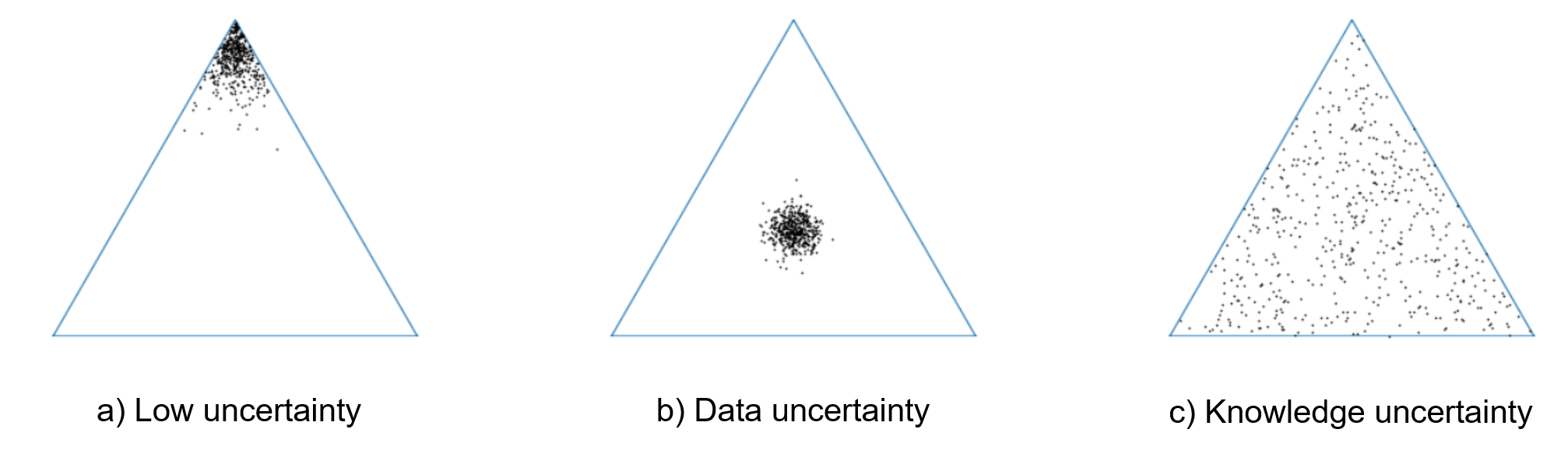] .bigger[ - 3-way classification task - each point represents the picture of ensemble member ] .citation[A. Malinin, Uncertainty Estimation in Deep Learning with application to Spoken Language Assessment, PhD Thesis 2019] --- exclude: true class: middle .grid[ .kol-6-12[ <br> <br> .center.width-80[] .caption[Reverend Bayes] ] .kol-6-12[ .center.width-60[] .caption[The Stig] ] ] .center.bigger[Inspiring theoreticians and high-performance seekers alike.*] .bottom.left.smaller[*Depending on the community, one method is frequently regarded as a special case for the other with different assumptions. Mind that Bayesian approaches and ensembles have different mindsets, however the two approaches often inspire each other. ] --- class: middle, center <!-- ## .bigger[Bayesian Neural Networks (BNNs)] --> # Bayesian Neural Networks (BNNs) --- class: middle .grid[ .kol-6-12[ .center.bold[Standard Neural Network] .center.width-80[] ] .kol-6-12[ .center.bold[Bayesian Neural Network] .center.width-80[] ] ] .grid[ .kol-6-12[ - Parameters represented by _single, fixed values (point estimates)_ - Conventional approaches to training NNs can be interpreted as _approximations_ to the full Bayesian method (equivalent to MLE or MAP estimation) ] .kol-6-12[ - Parameters represented by _distributions_ - For Gaussian prior: each parameter consists of a pair $(\mu, \sigma)$ describing a distribution over it (.red[2x more parameters]) ] ] .citation[C. Blundell et al., Weight Uncertainty in Neural Networks, ICML 2015] --- class: middle .bigger[Bayesian Neural Networks (BNNs) are *easy to formulate*, but **difficult** to perform inference in.] .bigger[Modern BNNs are trained with variational inference (_reparameterization trick_).] <!--.bigger[Modern BNNs are trained with variational inference (_reparameterization trick_) assuming parameter independence.] --> --- class: middle .center.width-70[] .caption[Standard Neural Network] $$p(\theta \mid \mathcal{D})$$ .hidden[ .grid[ .kol-6-12[ .right.width-10[] ] .kol-6-12[ .left.caption[Stochastic weights] ] ] .center[To train BNNs with variational inference we often assume parameter independence.] ] --- count: false class: middle .center.width-70[] .caption[Bayesian Neural Network] $$p(\theta \mid \mathcal{D}) = p(\theta\_1, \theta\_2, \theta\_3\mid \mathcal{D}) $$ .grid[ .kol-6-12[ .right.width-10[] ] .kol-6-12[ .left.caption[Stochastic weights] ] ] .hidden.center[To train BNNs with variational inference we often assume parameter independence.] --- count: false class: middle .center.width-70[] .caption[Bayesian Neural Network] $$p(\theta \mid \mathcal{D}) = p(\theta\_1, \theta\_2, \theta\_3\mid \mathcal{D})$$ .grid[ .kol-6-12[ .right.width-10[] ] .kol-6-12[ .left.caption[Stochastic weights] ] ] .center[To train BNNs with variational inference we often assume parameter independence.] --- class: middle, center ## Challenges of Bayesian Deep Learning .center.width-50[] --- ## Challenges of Bayesian Deep Learning - .bigger[Intractable posterior] .bigger[$\longrightarrow$ _posterior analysis, approximate posterior_ (.bold[Pavel])] .center.width-60[] --- count: false ## Challenges of Bayesian Deep Learning - .bigger[Intractable posterior] .bigger[$\longrightarrow$ _posterior analysis, approximate posterior_ (.bold[Pavel],.bold[Gianni])] - .bigger[Scalability to millions of parameters and large datasets] .bigger[$\longrightarrow$ _Laplace-Redux, subnetwork inference, large networks, ImageNet_ (.bold[Alexander],.bold[Gianni])] .grid[ .kol-6-12[ .center.width-100[] .caption[Last layer BNNs] ] .kol-6-12[ .center.width-100[] .caption[Subnetworks BNNs] ] ] --- count: false ## Challenges of Bayesian Deep Learning - .bigger[Intractable posterior] .bigger[$\longrightarrow$ _posterior analysis, approximate posterior_ (.bold[Pavel],.bold[Gianni])] - .bigger[Scalability to millions of parameters and large datasets] .bigger[$\longrightarrow$ _Laplace-Redux, subnetwork inference, large networks, ImageNet_ (.bold[Alexander],.bold[Gianni])] - .bigger[Suitability for complex tasks, e.g., computer vision] .bigger[$\longrightarrow$ _semantic segmentation, depth estimation_ (.bold[Gianni])] .center.width-70[] --- count: false ## Challenges of Bayesian Deep Learning - .bigger[Intractable posterior] .bigger[$\longrightarrow$ _posterior analysis, approximate posterior_ (.bold[Pavel],.bold[Gianni])] - .bigger[Scalability to millions of parameters and large datasets] .bigger[$\longrightarrow$ _Laplace-Redux, subnetwork inference, large networks, ImageNet_ (.bold[Alexander],.bold[Gianni])] - .bigger[Suitability for complex tasks, e.g., computer vision] .bigger[$\longrightarrow$ _semantic segmentation, depth estimation_ (.bold[Gianni])] - .bigger[Compatibility with modern deep learning practices] .bigger[$\longrightarrow$ $\texttt{TorchUncertainty}$ (.bold[Adrien])] .center.width-60[] --- class: middle .center.width-100[] --- layout: false class: end-slide, center count: false The end.