class: center, middle, title-slide count: false ### Deep Learning - MAP583 2019-2020 # Part 5: Transfer learning and Self-supervised learning .bold[Andrei Bursuc ] <br/> .width-10[] url: https://abursuc.github.io/slides/polytechnique/05_learning_tasks.html .citation[ With slides from A. Karpathy, F. Fleuret, G. Louppe, C. Ollion, O. Grisel, Y. Avrithis ...] --- # Outline ## Transfer learning ## Off-the shelf networks ## Fine-tuning ## (Task) transfer learning ## Multi-task learning ## Domain adaptation ## Self-supervised learning --- class: middle, center # Transfer Learning --- # Transfer learning - Assume two datasets $S$ and $T$ - Dataset $S$ is fully annotated, plenty of images and we can train a model $CNN_S$ on it - Dataset $T$ is not as much annotated and/or with fewer images + annotations of $T$ do not necessarily overlap with $S$ - We can use the model $CNN_S$ to learn a better $CNN_T$ - This is transfer learning --- # Transfer learning - Even if our dataset $T$ is not large, we can train a CNN for it - Pre-train a CNN on the dataset $S$ - The we can do: + fine-tuning + use CNN as feature extractor --- # Transfer learning Many flavors of transfer learning .center[<img src="images/part5/transfer_learning_taxonomy.png" style="width: 700px;" />] --- class: middle # Why using a pre-trained CNN (.italic[off-the-shelf]) would be a good idea? --- # Image ranking by CNN features .center.width-100[] - $3$-chanel RGB input, $224 \times 224$ - AlexNet pre-trained on ImageNet for classification .citation[A. Krizhevksy et al., Imagenet Classification with Deep Convolutional Neural Networks, NIPS 2012] --- count: false # Image ranking by CNN features .center.width-100[] - $3$-chanel RGB input, $224 \times 224$ - AlexNet pre-trained on ImageNet for classification - last fully connected layer ($fc\_6$): _global descriptor_ dimension $k=4096$ .citation[A. Krizhevksy et al., Imagenet Classification with Deep Convolutional Neural Networks, NIPS 2012] --- # VGG-16 .center[ <img src="images/part4/vgg.png" style="width: 600px;" /> ] .citation[K. Simonyan and A. Zisserman, Very deep convolutional networks for large-scale image recognition, NIPS 2014] --- # VGG-16 ```md Activation maps Parameters INPUT: [224x224x3] = 150K 0 CONV3-64: [224x224x64] = 3.2M (3x3x3)x64 = 1,728 CONV3-64: [224x224x64] = 3.2M (3x3x64)x64 = 36,864 POOL2: [112x112x64] = 800K 0 CONV3-128: [112x112x128] = 1.6M (3x3x64)x128 = 73,728 CONV3-128: [112x112x128] = 1.6M (3x3x128)x128 = 147,456 POOL2: [56x56x128] = 400K 0 CONV3-256: [56x56x256] = 800K (3x3x128)x256 = 294,912 CONV3-256: [56x56x256] = 800K (3x3x256)x256 = 589,824 CONV3-256: [56x56x256] = 800K (3x3x256)x256 = 589,824 POOL2: [28x28x256] = 200K 0 CONV3-512: [28x28x512] = 400K (3x3x256)x512 = 1,179,648 CONV3-512: [28x28x512] = 400K (3x3x512)x512 = 2,359,296 CONV3-512: [28x28x512] = 400K (3x3x512)x512 = 2,359,296 POOL2: [14x14x512] = 100K 0 CONV3-512: [14x14x512] = 100K (3x3x512)x512 = 2,359,296 CONV3-512: [14x14x512] = 100K (3x3x512)x512 = 2,359,296 CONV3-512: [14x14x512] = 100K (3x3x512)x512 = 2,359,296 POOL2: [7x7x512] = 25K 0 FC: [1x1x4096] = 4096 7x7x512x4096 = 102,760,448 FC: [1x1x4096] = 4096 4096x4096 = 16,777,216 FC: [1x1x1000] = 1000 4096x1000 = 4,096,000 TOTAL activations: 24M x 4 bytes ~= 93MB / image (x2 for backward) TOTAL parameters: 138M x 4 bytes ~= 552MB (x2 for plain SGD, x4 for Adam) ``` .credit[Slide credit: C. Ollion & O. Grisel] .citation[K. Simonyan and A. Zisserman, Very deep convolutional networks for large-scale image recognition, NIPS 2014] --- count: false # VGG-16 ```md Activation maps Parameters INPUT: [224x224x3] = 150K 0 CONV3-64: [224x224x64] = 3.2M (3x3x3)x64 = 1,728 CONV3-64: [224x224x64] = 3.2M (3x3x64)x64 = 36,864 POOL2: [112x112x64] = 800K 0 CONV3-128: [112x112x128] = 1.6M (3x3x64)x128 = 73,728 CONV3-128: [112x112x128] = 1.6M (3x3x128)x128 = 147,456 POOL2: [56x56x128] = 400K 0 CONV3-256: [56x56x256] = 800K (3x3x128)x256 = 294,912 CONV3-256: [56x56x256] = 800K (3x3x256)x256 = 589,824 CONV3-256: [56x56x256] = 800K (3x3x256)x256 = 589,824 POOL2: [28x28x256] = 200K 0 CONV3-512: [28x28x512] = 400K (3x3x256)x512 = 1,179,648 CONV3-512: [28x28x512] = 400K (3x3x512)x512 = 2,359,296 CONV3-512: [28x28x512] = 400K (3x3x512)x512 = 2,359,296 POOL2: [14x14x512] = 100K 0 CONV3-512: [14x14x512] = 100K (3x3x512)x512 = 2,359,296 CONV3-512: [14x14x512] = 100K (3x3x512)x512 = 2,359,296 CONV3-512: [14x14x512] = 100K (3x3x512)x512 = 2,359,296 POOL2: [7x7x512] = 25K 0 FC: [1x1x4096] = 4096 7x7x512x4096 = 102,760,448 *FC: [1x1x4096] = 4096 4096x4096 = 16,777,216 FC: [1x1x1000] = 1000 4096x1000 = 4,096,000 TOTAL activations: 24M x 4 bytes ~= 93MB / image (x2 for backward) TOTAL parameters: 138M x 4 bytes ~= 552MB (x2 for plain SGD, x4 for Adam) ``` .credit[Slide credit: C. Ollion & O. Grisel] .citation[K. Simonyan and A. Zisserman, Very deep convolutional networks for large-scale image recognition, NIPS 2014] --- # Image ranking by CNN features .center.width-70[] - query images .citation[A. Krizhevksy et al., Imagenet Classification with Deep Convolutional Neural Networks, NIPS 2012] --- count: false # Image ranking by CNN features .center.width-70[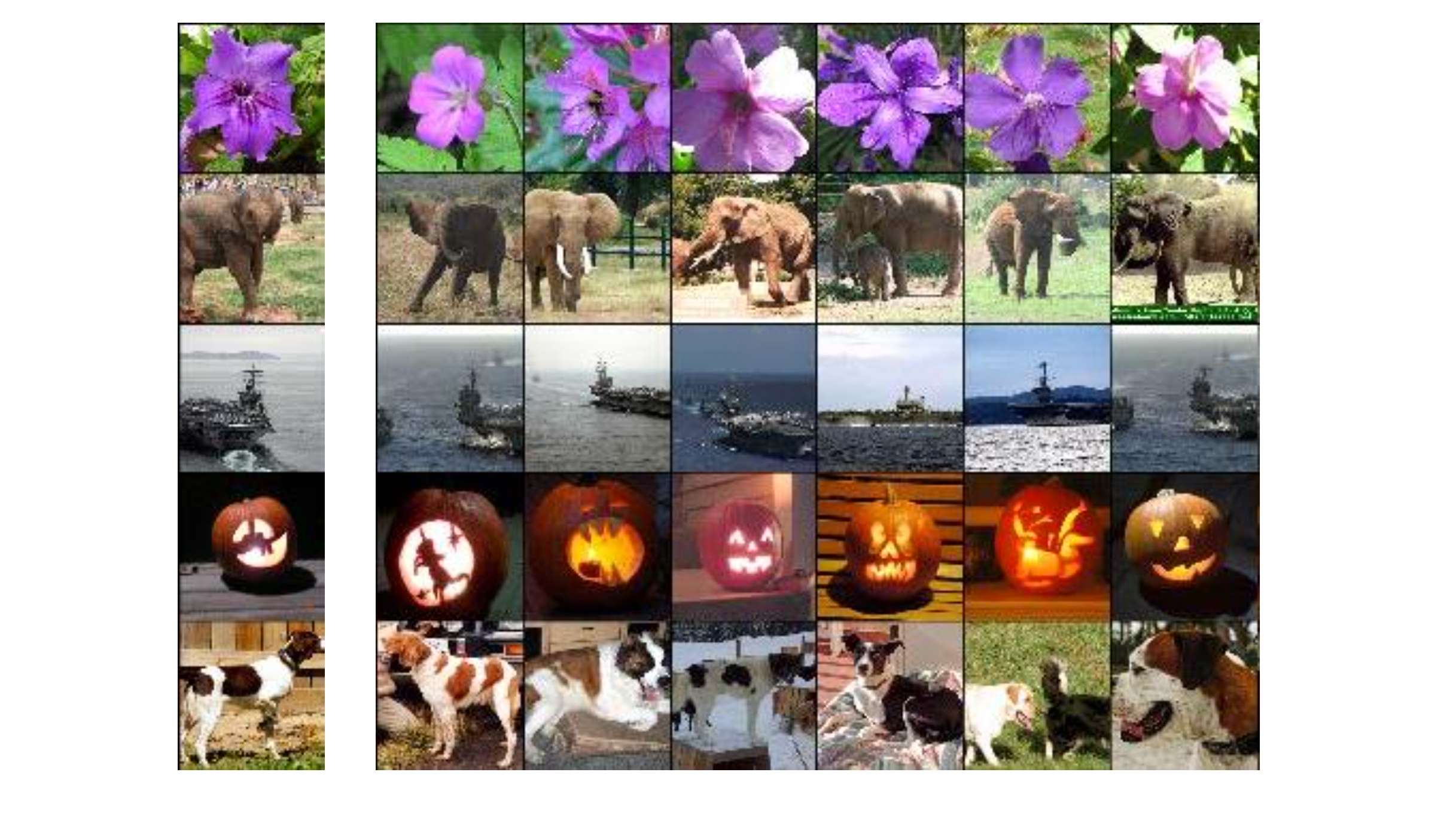] - query images : nearest neighbors in ImageNet according to Euclidean distance .citation[A. Krizhevksy et al., Imagenet Classification with Deep Convolutional Neural Networks, NIPS 2012] --- # Sampling information from feature maps .center.width-90[] - VGG-16 last convolutional layer, $k=512$ .citation[G. Tolias et al., Particular object retrieval with integral max-pooling, ICLR 2016] --- count: false # Sampling information from feature maps .center.width-90[] - VGG-16 last convolutional layer, $k=512$ - global spatial max-pooling/sum .citation[G. Tolias et al., Particular object retrieval with integral max-pooling, ICLR 2016] --- count: false # Sampling information from feature maps .center.width-90[] - VGG-16 last convolutional layer, $k=512$ - global spatial max-pooling/sum - $\ell\_2$ normalization, PCA-whitening, $\ell\_2$ normalization - _MAC_: maximum activation from convolutions .citation[G. Tolias et al., Particular object retrieval with integral max-pooling, ICLR 2016] --- count: false # VGG-16 ```md Activation maps Parameters INPUT: [224x224x3] = 150K 0 CONV3-64: [224x224x64] = 3.2M (3x3x3)x64 = 1,728 CONV3-64: [224x224x64] = 3.2M (3x3x64)x64 = 36,864 POOL2: [112x112x64] = 800K 0 CONV3-128: [112x112x128] = 1.6M (3x3x64)x128 = 73,728 CONV3-128: [112x112x128] = 1.6M (3x3x128)x128 = 147,456 POOL2: [56x56x128] = 400K 0 CONV3-256: [56x56x256] = 800K (3x3x128)x256 = 294,912 CONV3-256: [56x56x256] = 800K (3x3x256)x256 = 589,824 CONV3-256: [56x56x256] = 800K (3x3x256)x256 = 589,824 POOL2: [28x28x256] = 200K 0 CONV3-512: [28x28x512] = 400K (3x3x256)x512 = 1,179,648 CONV3-512: [28x28x512] = 400K (3x3x512)x512 = 2,359,296 CONV3-512: [28x28x512] = 400K (3x3x512)x512 = 2,359,296 POOL2: [14x14x512] = 100K 0 CONV3-512: [14x14x512] = 100K (3x3x512)x512 = 2,359,296 CONV3-512: [14x14x512] = 100K (3x3x512)x512 = 2,359,296 CONV3-512: [14x14x512] = 100K (3x3x512)x512 = 2,359,296 *POOL2: [7x7x512] = 25K 0 FC: [1x1x4096] = 4096 7x7x512x4096 = 102,760,448 FC: [1x1x4096] = 4096 4096x4096 = 16,777,216 FC: [1x1x1000] = 1000 4096x1000 = 4,096,000 TOTAL activations: 24M x 4 bytes ~= 93MB / image (x2 for backward) TOTAL parameters: 138M x 4 bytes ~= 552MB (x2 for plain SGD, x4 for Adam) ``` .credit[Slide credit: C. Ollion & O. Grisel] .citation[K. Simonyan and A. Zisserman, Very deep convolutional networks for large-scale image recognition, NIPS 2014] --- # Global max-pooling: matching .center.width-50[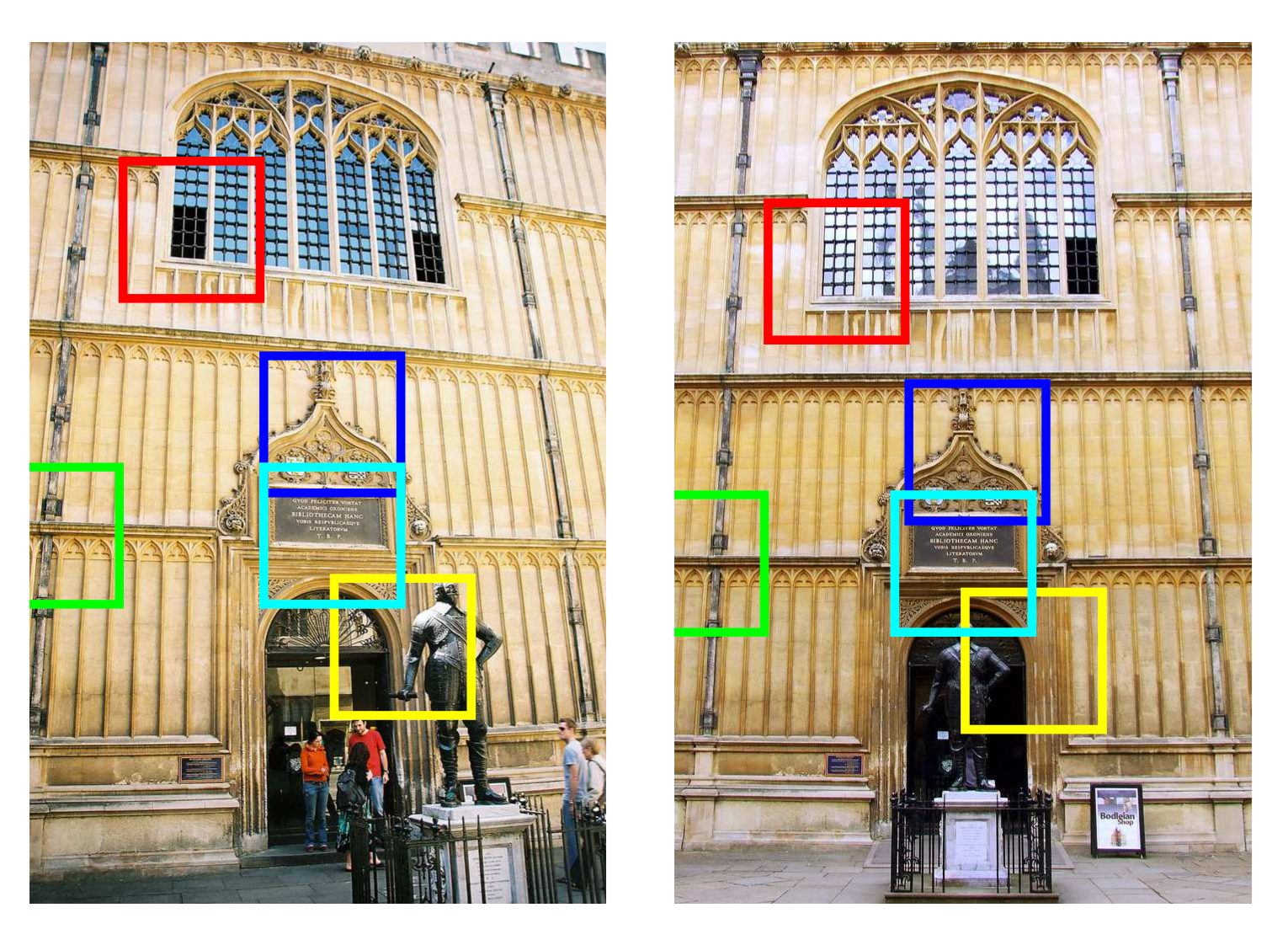] - receptive fields of 5 components of MAC vectors that contribute most to image similarity .citation[G. Tolias et al., Particular object retrieval with integral max-pooling, ICLR 2016] --- # Global max-pooling: matching .center.width-90[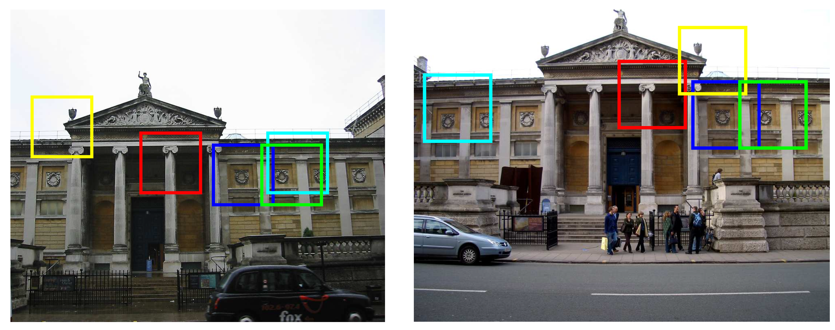] - receptive fields of 5 components of MAC vectors that contribute most to image similarity .citation[G. Tolias et al., Particular object retrieval with integral max-pooling, ICLR 2016] --- # Global max-pooling: matching .center.width-60[] - receptive fields of 5 components of MAC vectors that contribute most to image similarity .citation[G. Tolias et al., Particular object retrieval with integral max-pooling, ICLR 2016] --- # Regional max-pooling (R-MAC) .center.width-90[] - VGG-16 last convolutional layer, $k=512$ - fixed mulitscale overlapping regions .citation[G. Tolias et al., Particular object retrieval with integral max-pooling, ICLR 2016] --- count: false # Regional max-pooling (R-MAC) .center.width-90[] - VGG-16 last convolutional layer, $k=512$ - fixed mulitscale overlapping regions, spatial _max_-pooling .citation[G. Tolias et al., Particular object retrieval with integral max-pooling, ICLR 2016] --- count: false # Regional max-pooling (R-MAC) .center.width-90[] - VGG-16 last convolutional layer, $k=512$ - fixed mulitscale overlapping regions, spatial _max_-pooling - $\ell\_2$ normalization, PCA-whitening, $\ell\_2$ normalization .citation[G. Tolias et al., Particular object retrieval with integral max-pooling, ICLR 2016] --- count: false # Regional max-pooling (R-MAC) .center.width-90[] - VGG-16 last convolutional layer, $k=512$ - fixed mulitscale overlapping regions, spatial _max_-pooling - $\ell\_2$ normalization, PCA-whitening, $\ell\_2$ normalization - _sum_-pooling over all descriptors, $\ell\_2$ normalization .citation[G. Tolias et al., Particular object retrieval with integral max-pooling, ICLR 2016] --- class: middle # Can we do more with a bit of training? --- class: middle Training a task-specific linear classifier on top of CNN features led to SoTA or nearly-SoTA results .center.width-80[] .citation[A. Razavian et al., CNN Features off-the-shelf: an Astounding Baseline for Recognition, arXiv 2014] --- # Tasks and datasets ### Object classification and detection .center.width-80[] .caption[Pascal VOC] ### Fine grained classification .center.width-40[] .caption[CUB 200 2011] --- # Tasks and datasets ### Instance retrieval .center.width-100[] .caption[Oxford Buildings and Paris Buildings] --- <br/><br/><br/><br/> .center.width-60[] -- count: false ##.center[.red[2020 edit: Not quite there yet]] --- class: middle, center # Fine-tuning --- # Fine-tuning - Assume the parameters of $CNN_S$ are already a good start near our final local optimum - Use them as the initial parameters for our new CNN for the target dataset - This is a good solution when the dataset $T$ is relatively big + e.g. for Imagenet $S$ with 1M images, $T$ with a few thousands images --- # Fine-tuning .center[<img src="images/part5/finetuning.png" style="width: 600px;" />] - Depending on the size of $T$ decide which layer to freeze and which to finetune/replace - Use lower learning rate when fine-tuning: about $\frac{1}{10}$ of original learning rate + for new layers use agressive learning rate - If $S$ and $T$ are very similar,fine-tune only fully-connected layers - If datasets are different and you have enough data, fine-tune all layers --- # Selecting which layers to freeze .left-column[ <br/> .center[Visualize highly exciting patterns across layers] ] .right-column[.center[<img src="images/part5/deep_pipeline_5.png" height="120px">]] .reset-column[ ] .center.width-70[] .citation[M. Zeiler & R. Fergus, Visualizing and Understanding Convolutional Networks, ECCV 2014] --- # Fine-tuning a ResNet? .center.width-100[] --- count: false # Fine-tuning a ResNet? .center.width-100[] Preferably select layers to freeze main block .center.width-70[] --- class: middle .center.width-60[] Pre-trained networks are the bread and butter in computer vision (at large) solutions, both academic and industrial. Other communities are starting to follow this practice. --- class: middle Pre-trained networks are the bread and butter in computer vision: _semantic segmentation_ .grid[ .kol-6-12[ .center[] .caption[SegNet] .center[] .caption[DeepLabV3] ] .kol-6-12[ .center[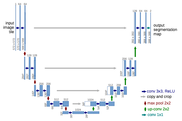] .caption[U-Net] .center[] .caption[PSPNet] ] ] --- class: middle Pre-trained networks are the bread and butter in computer vision: _object retrieval_ .center.width-90[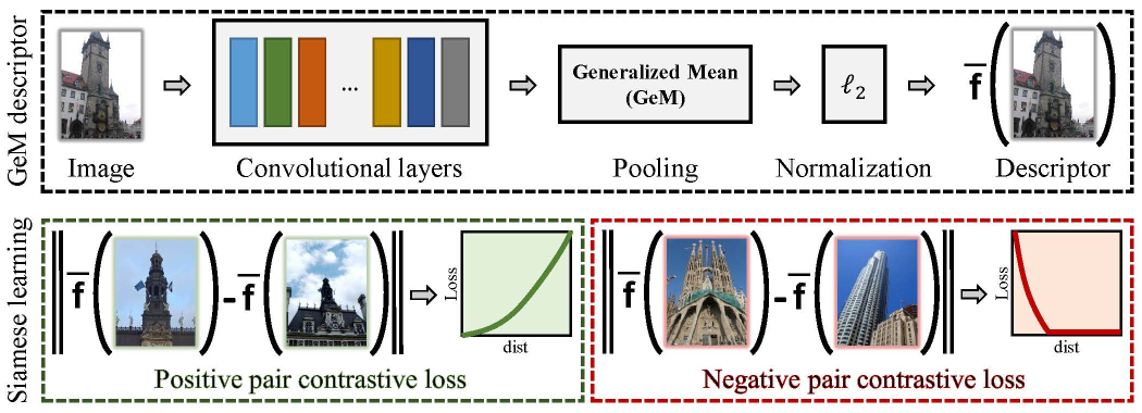] .citation[F. Radenovic, CNN Image Retrieval Learns from BoW: Unsupervised Fine-Tuning with Hard Examples, ECCV 2016] --- class: middle Pre-trained networks are the bread and butter in computer vision: _visual question answering_ .center.width-90[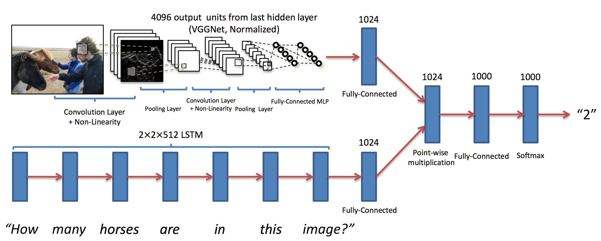] .caption[VQA] .citation[A. Agrawal et al., VQA: Visual Question Answering, ICCV 2015] --- Pre-trained networks are the bread and butter in computer vision: _style transfer_ .center[ <video width="640" height="480" controls loop> <source src="images/part5/picasso-periods.mp4" type="video/mp4"> </video> ] --- Pre-trained networks are the bread and butter in computer vision: _style transfer_ .center.width-80[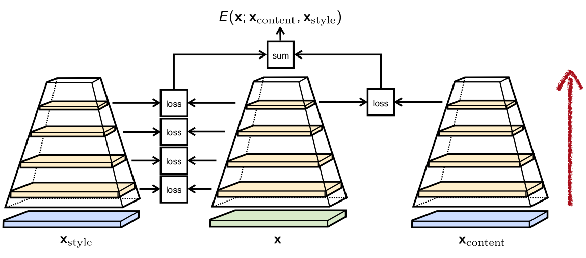] .citation[L. Gatys et al., A Neural Algorithm of Artistic Style, arXiv 2015] --- class: middle, center # .green[Question ?] --- class: middle Imagine you have to work with x-ray images and you don't have too much of it. _What can you do?_ .center.width-70[] --- class: middle There is a popular belief that pre-training is always better than random initialization even after convergence. --- count: false class: middle There is a popular belief that ~~pre-training is always better than random initialization even after convergence~~. ## .center[.red[False / Not anymore at least]] --- # Rethinking pre-training .left-column[ .center.width-80[] ] .right-column[ .center.width-100[] ] .citation[K. He et al., Rethinking ImageNet Pre-training, arXiv 2018 ] --- class: middle, center # (Task) Transfer learning --- class: middle # Taskonomy: Disentangling Task Transfer Learning .citation[A. Zamir et al., Taskonomy: Disentangling Task Transfer Learning, CVPR 2018] --- # Question - Some vision tasks are more inter-related than others: + depth estimation could help surface normals estimation? + scene layout could help object detection? - for some task annotation data can be more easily obtainable than others - could we find fully computational approach for modeling the structure of the space of visual tasks? .citation[A. Zamir et al., Taskonomy: Disentangling Task Transfer Learning, CVPR 2018] --- # Task bank/dictionary .grid[ .kol-6-12[ - Task Bank + 26 semantic, 2d, 3d and other tasks - Dataset + 4M real images + each image has the GT label for all tasks - Task specific networks + 26 x ] .kol-6-12[ .center[<img src="images/part5/task_dictionary.png" style="width: 400px;" />] ] ] --- # Task bank/dictionary .center[<iframe width="900" height="495" src="https://www.youtube.com/embed/SUq1CiX-KzM" frameborder="0" allow="autoplay; encrypted-media" allowfullscreen></iframe>] .citation[A. Zamir et al., Taskonomy: Disentangling Task Transfer Learning, CVPR 2018] --- # Common architecture .center[<img src="images/part5/taskonomy_architecture.png" style="width: 650px;" />] - encoder: ResNet50 - transfer function: 2 conv layers - decoder: 15 _fully convolutional_ layers / 2-3 _fully connected_ layers .citation[A. Zamir et al., Taskonomy: Disentangling Task Transfer Learning, CVPR 2018] --- # Common architecture .center[<img src="images/part5/taskonomy_architecture.png" style="width: 650px;" />] - _full training_ (gold standard): $120k$ training, $16k$ validation, $17k$ testing - _fine-tuning_: $1 - 16k$ .citation[A. Zamir et al., Taskonomy: Disentangling Task Transfer Learning, CVPR 2018] --- # Computational model .center.width-100[] .citation[A. Zamir et al., Taskonomy: Disentangling Task Transfer Learning, CVPR 2018] --- # Computed taxonomies .center[<img src="images/part5/taskonomy_computed_taxonomies.png" style="width: 800px;" />] .citation[A. Zamir et al., Taskonomy: Disentangling Task Transfer Learning, CVPR 2018] --- --- class: middle, center # Multi-Task Learning --- class: middle .big[If we have different types of labels for a given dataset we can: - train multiple models (one for each type of labels) - inject all knowledge in a single model] --- count: false class: middle .big[If we have different types of labels for a given dataset we can: - train multiple models (one for each type of labels) - __inject all knowledge in a single model__] --- # Multi-Task Learning .center.width-100[] --- count: false # Multi-Task Learning .center.width-80[] .big[$$ \mathcal{L}\_{total} = \sum\_i w\_i \mathcal{L}\_i$$] .big[$$ \sum\_i w\_i = 1$$] --- class: middle, center # Domain Adaptation --- # Example: Internet images $\rightarrow$ webcam .center.width-80[] --- # Example: (semi-)synthetic $\rightarrow$ real .left-column[ .center.width-70[] ] .right-column[ .center.width-70[] ] --- # Domain-adversarial networks .center.width-100[] .citation[Y. Ganin et al., Domain-Adversarial Training of Neural Networks, JMLR 2016] --- # Domain-adversarial networks .center.width-60[] - build a network - train .green[feature extractor] + .blue[class predictor] on source data - train .green[feature extractor] + .pink[domain classifier] on source+target data - use .green[feature extractor] + .blue[class predictor] at test time .citation[Y. Ganin et al., Domain-Adversarial Training of Neural Networks, JMLR 2016] --- # Domain-adversarial networks .center.width-100[] - build a network - train .green[feature extractor] + .blue[class predictor] on source data - train .green[feature extractor] + .pink[domain classifier] on source+target data - use .green[feature extractor] + .blue[class predictor] at test time .citation[Y. Ganin et al., Domain-Adversarial Training of Neural Networks, JMLR 2016] --- # Large-gap domain adaptation Using video games to generate training data .center.width-70[] .caption[GTA V] .citation[S. Richter et al., Playing for Data: Ground Truth from Computer Games, ECCV 2016] --- # Unsupervised domain adaptation .center.width-50[] .caption[Directly testing on the target data is not quite optimal] .citation[T. Vu et al., ADVENT: Adversarial Entropy Minimization for Domain Adaptation in Semantic Segmentation, CVPR 2019] --- # Unsupervised domain adaptation .center.width-90[] .caption[ADVENT - Adversarial Entropy Minimization for Domain Adaptation] .citation[T. Vu et al., ADVENT: Adversarial Entropy Minimization for Domain Adaptation in Semantic Segmentation, CVPR 2019] --- # Unsupervised domain adaptation .center.width-60[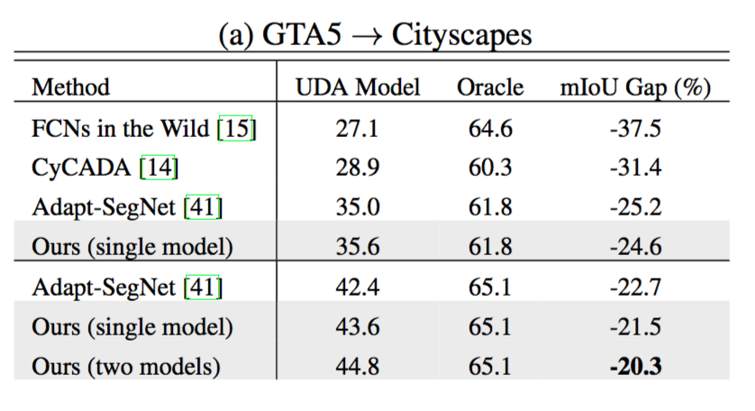] .caption[GAP w.r.t. oracle, .italic[i.e.] when training on the target data] .citation[T. Vu et al., ADVENT: Adversarial Entropy Minimization for Domain Adaptation in Semantic Segmentation, CVPR 2019] --- # Unsupervised domain adaptation .center.width-80[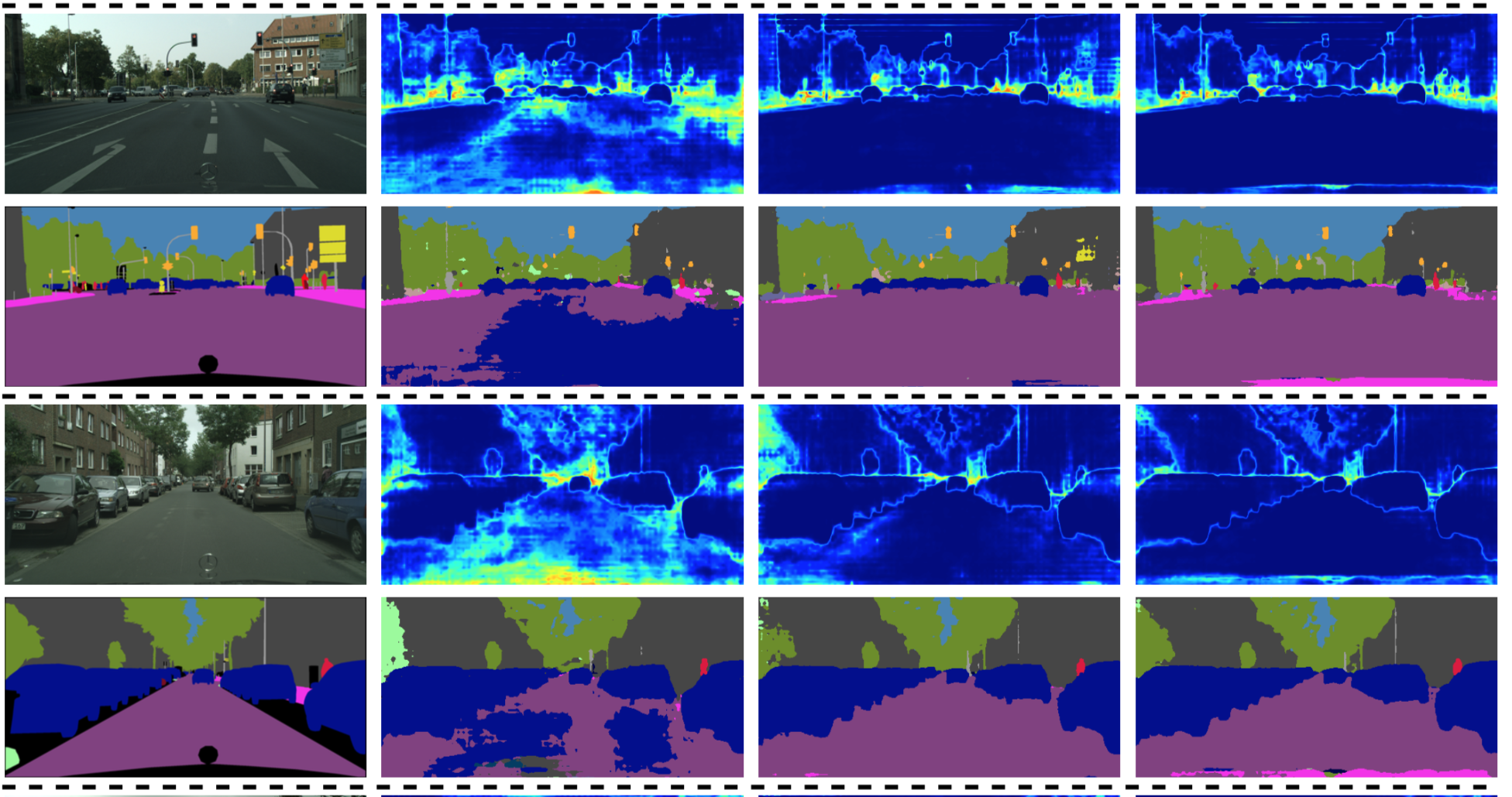] .caption[Semantic segmentation: from GTA V $\rightarrow$ Cityscapes] .citation[T. Vu et al., ADVENT: Adversarial Entropy Minimization for Domain Adaptation in Semantic Segmentation, CVPR 2019] --- # Unsupervised domain adaptation .center.width-80[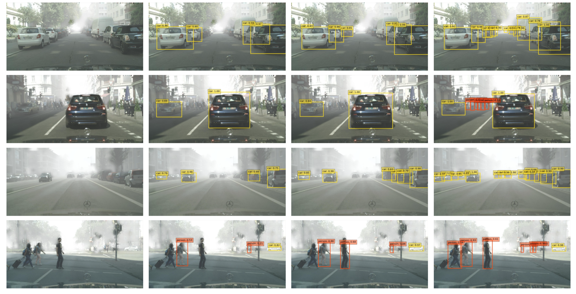] .caption[Object detection: from Cityscapes $\rightarrow$ Foggy Cityscapes (synthetic fog)] .citation[T. Vu et al., ADVENT: Adversarial Entropy Minimization for Domain Adaptation in Semantic Segmentation, CVPR 2019] --- # Also domain adaptation Instead of learning domain invariant features, we can modify the synthetic data to "look" more realistic. .center.width-60[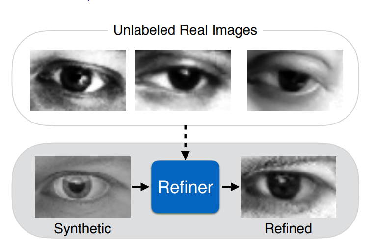] .citation[A. Srivastava et al., Learning from Simulated and Unsupervised Images through Adversarial Training, CVPR 2017] --- # Also domain adaptation .center.width-100[] .citation[A. Srivastava et al., Learning from Simulated and Unsupervised Images through Adversarial Training, CVPR 2017] --- count: false # Also domain adaptation .center.width-100[] .center.width-80[] .citation[A. Srivastava et al., Learning from Simulated and Unsupervised Images through Adversarial Training, CVPR 2017] --- class: middle, center # Self-supervised learning --- # Self-supervised learning Self-supervised learning consists of two learning stages: - 1) Learn a feature extractor with a proxy annotation-free task - 2) Transfer it to an end task: + end tasks: image classification, object detection, etc. - __Goal__: at 1st stage learn good features for the 2nd stage .center.width-90[] --- class: middle, center ## Self-supervised learning is the platypus of machine learning .center.width-70[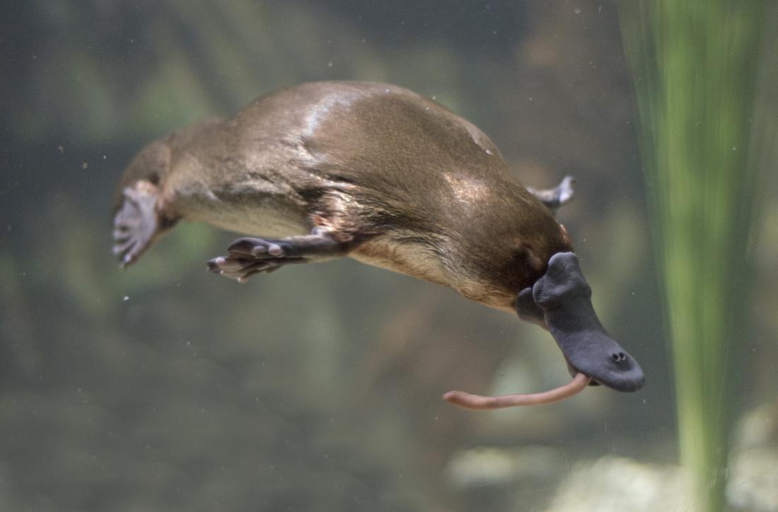] --- class: middle ## .center[Self-supervised learning is the platypus of machine learning] .center.width-50[] - the loss is supervised - no labeling is needed since labeling comes from the data itself - it's somewehere in-between _supervised_ and _unsupervised learning_ --- # Image colorization .center.width-60[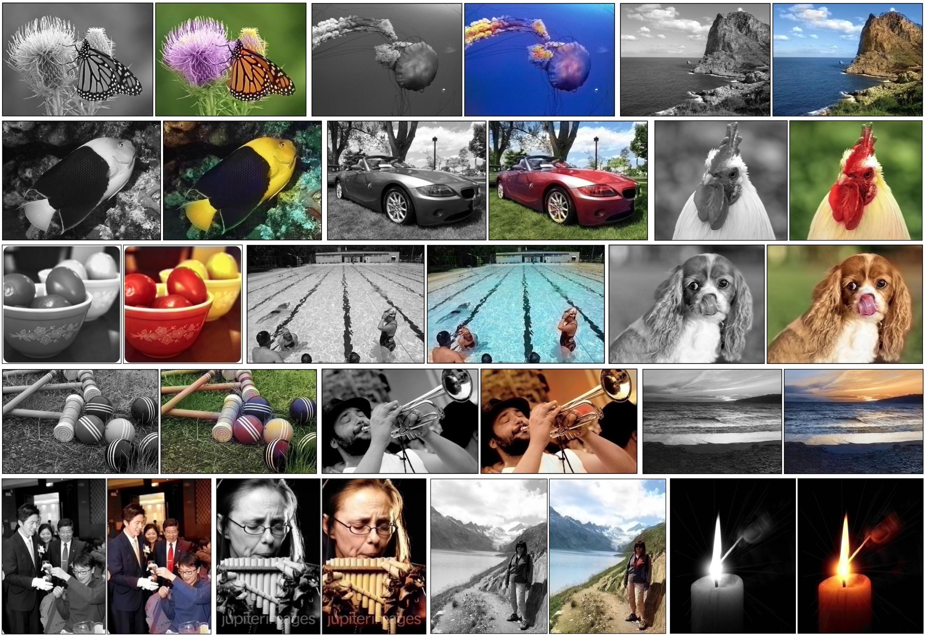] .caption[Convert grayscale images to colorized] .citation[R. Zhang et al., Colorful image colorization, ECCV 2016] --- # Image colorization <br/> <br/> <br/> .center.width-100[] .citation[R. Zhang et al., Colorful image colorization, ECCV 2016] --- # Exemplar networks - perturb image patches (color distorsions, cropping, affine transformations) - train net to classify exemplars as same class .center.width-80[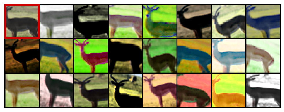] .citation[A. Dosovitskiy et al., Discriminative Unsupervised Feature Learning with Exemplar Convolutional Neural Networks, PAMI 2015] --- # Rotation prediction <br/> <br/> <br/> .center.width-80[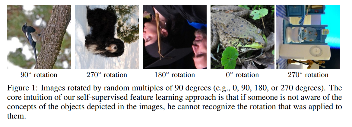] .citation[S. Gidaris et al., Unsupervised representation learning by predicting image rotations, ICLR 2018] --- # Rotation prediction .center.width-80[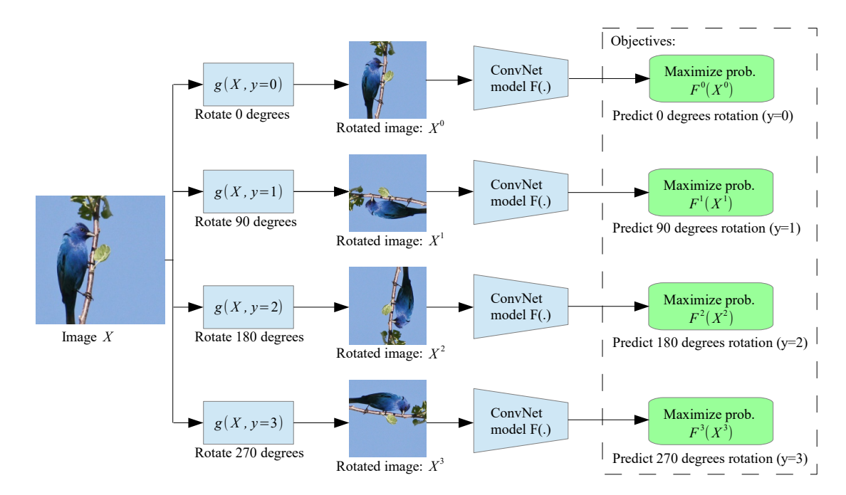] .citation[S. Gidaris et al., Unsupervised representation learning by predicting image rotations, ICLR 2018] --- # Relative patch location .center.width-100[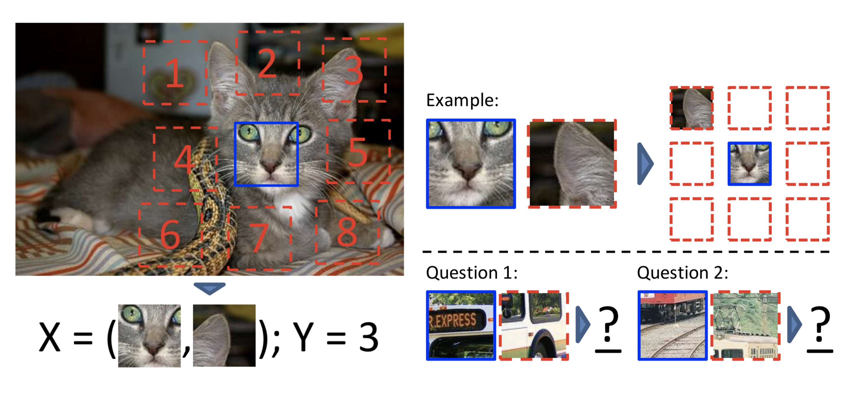] .citation[C. Doersch et al., Unsupervised Visual Representation Learning by Context Prediction, ICCV 2015] --- # Relative patch location .center.width-100[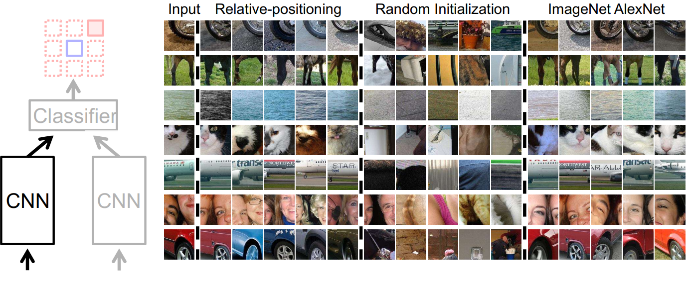] .citation[C. Doersch et al., Unsupervised Visual Representation Learning by Context Prediction, ICCV 2015] --- # Jigsaw puzzles .center.width-100[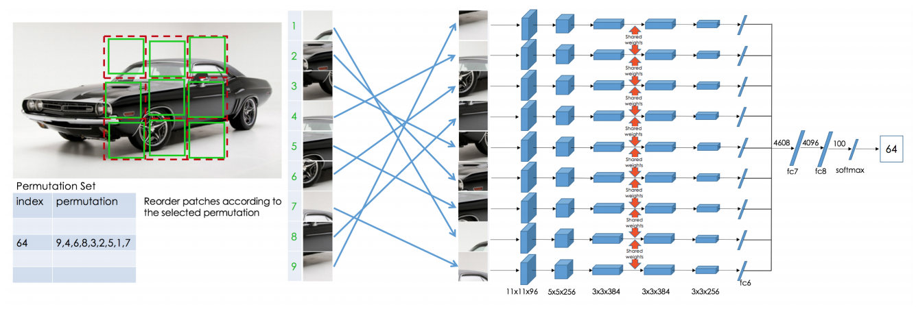] .citation[M. Noroozi and P. Favaro, Unsupervised Learning of Visual Representations by Solving Jigsaw Puzzles, ECCV 2016] --- # Context encoders .center.width-80[] .citation[D. Pathak, Context Encoders: Feature Learning by Inpainting, CVPR 2016] --- # Context encoders .center.width-80[] .citation[D. Pathak, Context Encoders: Feature Learning by Inpainting, CVPR 2016] --- # Predicting the correct order of time .center.width-50[] .citation[I. Misra et al., Shuffle and Learn: Unsupervised Learning using Temporal Order Verification, ECCV 2016] --- # Predicting the correct order of time .center.width-60[] .citation[I. Misra et al., Shuffle and Learn: Unsupervised Learning using Temporal Order Verification, ECCV 2016] --- # Sorting video sequences .center.width-70[] .citation[H.Y. Lee et al., Unsupervised Representation Learning by Sorting Sequences, ICCV 2017] --- # Sorting video sequences .center.width-80[] .citation[H.Y. Lee et al., Unsupervised Representation Learning by Sorting Sequences, ICCV 2017] --- # Audio-visual correspondence <br/> <br/> ## .center[ Can audio and video learn from each other?] .center.width-80[] .citation[R. Arandjelovic, Look, Listen and Learn, ICCV 2017] .credit[Slide credit: A. Zissermanl] --- #Audio-visual correspondence .center.width-80[] .citation[R. Arandjelovic, Look, Listen and Learn, ICCV 2017] .credit[Slide credit: A. Zissermanl] --- #Audio-visual correspondence .center.width-80[] .citation[R. Arandjelovic, Look, Listen and Learn, ICCV 2017] .credit[Slide credit: A. Zissermanl] --- #Audio-visual correspondence .center.width-80[] .citation[R. Arandjelovic, Look, Listen and Learn, ICCV 2017] .credit[Slide credit: A. Zissermanl] --- #Audio-visual correspondence .center.width-90[] .citation[R. Arandjelovic, Look, Listen and Learn, ICCV 2017] .credit[Slide credit: A. Zissermanl] --- #Audio-visual correspondence .center.width-80[] .citation[R. Arandjelovic, Look, Listen and Learn, ICCV 2017] --- #Audio-visual correspondence .center.width-80[] .citation[R. Arandjelovic, Look, Listen and Learn, ICCV 2017] --- # Contrastive representations .grid[ .kol-6-12[ .center.width-80[] ].kol-6-12[ ] ] Learn to recognize perturbed variants of the same image .citation[I. Misra, Self-Supervised Learning of Pretext-Invariant Representations, arXiv 2018] --- count: false # Contrastive representations .grid[ .kol-6-12[ .center.width-80[] ].kol-6-12[ .center.width-80[] ] ] Learn to recognize perturbed variants of the same image. We're starting to finally outperform ImageNet supervised pre-trained models. .citation[I. Misra, Self-Supervised Learning of Pretext-Invariant Representations, arXiv 2018] --- class: middle, center .center.width-40[] --- class: middle, center .center.width-90[] --- class: middle, center .center.width-90[] --- # Practical utilisation of self-supervision Extract knowledge from unlabeled data using self-supervision in a multi-task learning pipeline .center.width-100[] .citation[S. Gidaris et al., Boosting Few-Shot Visual Learning with Self-Supervision, ICCV 2019] --- # Practical utilisation of self-supervision Extract knowledge from unlabeled data using self-supervision in a multi-task learning pipeline .center.width-100[] .citation[F.M. Carlucci, Domain Generalization by Solving Jigsaw Puzzles, CVPR 2019] --- # Today ## Transfer learning ## Off-the shelf networks ## Fine-tuning ## (Task) transfer learning ## Multi-task learning ## Domain adaptation ## Self-supervised learning --- class: end-slide, center count: false The end.