class: center, middle ### Deep Learning - MAP583 2019-2020 ## Part 6: Under the hood .bold[Andrei Bursuc ] <br/> .width-10[] url: https://abursuc.github.io/slides/polytechnique/06_under_hood.html .citation[ With slides from A. Karpathy, F. Fleuret, J. Johnson, S. Yeung, G. Louppe, Y. Avrithis ...] --- class: center, middle # GPUs .center[<img src="images/part6/nvidia_titan_xp.jpg" style="width: 700px;" />] --- # CPU vs GPU <br/> .left[ .center[CPU] <br/> .center[<img src="images/part6/cpu.png" style="width: 350px;" />] ] .right[ .center[GPU] <br/> .center[<img src="images/part6/nvidia_tesla_v100.jpg" style="width: 500px;" />] ] --- # CPU vs GPU .left-column[ - CPU: + fewer cores; each core is faster and more powerful + useful for sequential tasks ] .right-column[ - GPU: + more cores; each core is slower and weaker + great for parallel tasks ] .reset-column[] .center[<img src="images/part6/cpu_vs_gpu_2.png" style="width: 650px;" />] --- # CPU vs GPU .left-column[ - CPU: + fewer cores; each core is faster and more powerful + useful for sequential tasks ] .right-column[ - GPU: + more cores; each core is slower and weaker + great for parallel tasks ] .reset-column[] .center[<img src="images/part6/cpu_vs_gpu_1.png" style="width: 650px;" />] .credit[Figure credit: J. Johnson] --- # CPU vs GPU - SP = single precision, 32 bits / 4 bytes - DP = double precision, 64 bits / 8 bytes .center[<img src="images/part6/cpu_vs_gpu_3.png" style="width: 700px;" />] --- # CPU vs GPU .center[<img src="images/part6/gpu_benchmark.png" style="width: 700px;" />] .citation[Benchmarking State-of-the-Art Deep Learning Software Tools, Shi et al., 2016] --- # CPU vs GPU - more benchmarks available at [https://github.com/jcjohnson/cnn-benchmarks](https://github.com/jcjohnson/cnn-benchmarks) .center[<img src="images/part6/cpu_vs_gpu_4.png" style="width: 700px;" />] .credit[Figure credit: J. Johnson] --- count: false # CPU vs GPU - more benchmarks available at [https://github.com/jcjohnson/cnn-benchmarks](https://github.com/jcjohnson/cnn-benchmarks) .center[<img src="images/part6/cpu_vs_gpu_5.png" style="width: 700px;" />] .credit[Figure credit: J. Johnson] --- # System .center[<img src="images/part6/system_1.png" style="width: 700px;" />] .credit[Figure credit: F. Fleuret] --- count: false # System .center[<img src="images/part6/system_2.png" style="width: 700px;" />] .credit[Figure credit: F. Fleuret] --- count: false # System .center[<img src="images/part6/system_3.png" style="width: 700px;" />] .credit[Figure credit: F. Fleuret] --- count: false # System .center[<img src="images/part6/system_4.png" style="width: 700px;" />] .credit[Figure credit: F. Fleuret] --- count: false # System .center[<img src="images/part6/system_5.png" style="width: 700px;" />] .credit[Figure credit: F. Fleuret] --- count: false # System .center[<img src="images/part6/system_6.png" style="width: 700px;" />] .credit[Figure credit: F. Fleuret] --- count: false # System .center[<img src="images/part6/system_7.png" style="width: 700px;" />] .credit[Figure credit: F. Fleuret] --- # GPU - NVIDIA GPUs are programmed through CUDA (.purple[Compute Unified Device Architecture]) - The alternative is OpenCL, supported by several manufacturers but with significant less investments than Nvidia - Nvidia and CUDA are dominating the field by far, though some alternatives start emerging: Google TPUs, embedded devices. --- # Libraries - BLAS (_Basic Linear Algebra Subprograms_): vector/matrix products, and the cuBLAS implementation for NVIDIA GPUs - LAPACK (_Linear Algebra Package_): linear system solving, Eigen-decomposition, etc. - cuDNN (_NVIDIA CUDA Deep Neural Network library_) computations specific to deep-learning on NVIDIA GPUs. --- # GPU usage in pytorch - Tensors of torch.cuda types are in the GPU memory. Operations on them are done by the GPU and resulting tensors are stored in its memory. - Operations cannot mix different tensor types (CPU vs. GPU, or different numerical types); except `copy_()` - Moving data between the CPU and the GPU memories is far slower than moving it inside the GPU memory. --- # GPU usage in pytorch - The `Tensor` method `cuda()` / `.to('cuda')` returns a clone on the GPU if the tensor is not already there or returns the tensor itself if it was already there, keeping the bit precision. - The method `cpu()` / `.to('cpu')` makes a clone on the CPU if needed. - They both keep the original tensor unchanged --- class: center, middle # Understanding and visualizing CNNs .center[ <img src="images/part6/cnn_js.png" style="width: 700px;" /> ] --- # What happens inside a CNN? .left-column[ <br/> .center[Visualize first layers filters/weights] ] .right-column[.center[<img src="images/part6/deep_pipeline_1.png" height="120px">]] .reset-column[] .center[<img src="images/part6/cnn_vis_1.png" style="width: 600px;"> ] .citation[M. Zeiler & R. Fergus, Visualizing and Understanding Convolutional Networks, ECCV 2014] --- count: false # What happens inside a CNN? .left-column[ <br/> .center[Visualize first layers filters/weights] ] .right-column[.center[<img src="images/part6/deep_pipeline_1.png" height="120px">]] .reset-column[ ] .left[<img src="images/part6/cnn_vis_2.png" style="width: 100px;"> ] .citation[M. Zeiler & R. Fergus, Visualizing and Understanding Convolutional Networks, ECCV 2014] --- count: false # What happens inside a CNN? .left-column[ - Visualize behavior in higher layers - We can visualize filters at higher layers, but they are less intuitive ] .right-column[.center[<img src="images/part6/deep_pipeline_3.png" height="120px">]] .reset-column[ ] <br/> .center[<img src="images/part6/cnn_vis_7.png" style="width: 450px;"> ] --- count: false # What happens inside a CNN? .left-column[ <br/> .center[Visualize first layers filters/weights] ] .right-column[.center[<img src="images/part6/deep_pipeline_2.png" height="120px">]] .reset-column[ ] .left[<img src="images/part6/cnn_vis_3.png" style="height: 300px;"> ] .citation[M. Zeiler & R. Fergus, Visualizing and Understanding Convolutional Networks, ECCV 2014] --- count: false # What happens inside a CNN? .left-column[ <br/> .center[Visualize first layers filters/weights] ] .right-column[.center[<img src="images/part6/deep_pipeline_3.png" height="120px">]] .reset-column[ ] .left[<img src="images/part6/cnn_vis_4.png" style="height: 300px;"> ] .citation[M. Zeiler & R. Fergus, Visualizing and Understanding Convolutional Networks, ECCV 2014] --- count: false # What happens inside a CNN? .left-column[ <br/> .center[Visualize first layers filters/weights] ] .right-column[.center[<img src="images/part6/deep_pipeline_4.png" height="120px">]] .reset-column[ ] .left[<img src="images/part6/cnn_vis_5.png" style="height: 400px;"> ] .citation[M. Zeiler & R. Fergus, Visualizing and Understanding Convolutional Networks, ECCV 2014] --- count: false # What happens inside a CNN? .left-column[ <br/> .center[Visualize first layers filters/weights] ] .right-column[.center[<img src="images/part6/deep_pipeline_5.png" height="120px">]] .reset-column[ ] .left[<img src="images/part6/cnn_vis_6.png" style="height: 400px;"> ] .citation[M. Zeiler & R. Fergus, Visualizing and Understanding Convolutional Networks, ECCV 2014] --- count: false # What happens inside a CNN? .left-column[ - 4096d "signature" for an image (layer right before the classifier) - Visualize with t-SNE: [here](http://cs.stanford.edu/people/karpathy/cnnembed/) ] .right-column[.center[<img src="images/part6/deep_pipeline_6.png" height="120px">]] .reset-column[ ] .center[<img src="images/part6/cnn_vis_8.png" style="height: 370px;"> ] --- # Feature evolution during training - For a particular neuron (that generates a feature map) - Pick the strongest activation during training - For epochs 1, 2, 5, 10, 20, 30, 40, 64 <br> .center[<img src="images/part6/feature_evolution.png" style="width: 1000px;"> ] .citation[M. Zeiler & R. Fergus, Visualizing and Understanding Convolutional Networks, ECCV 2014] --- # Some words of caution These specific neurons firing on specific patterns or classes, .italic[i.e.] _cat-neurons_ might give us the idea of understanding the behavior of neural networks. -- count: false However, recent results show that removing these neurons, the performance of the networks does not decrease noticably. .center.width-60[] .citation[A. Morcos et al., On the importance of single directions for generalization, ICLR 2018] --- # Visualize layer activations/feature maps ## AlexNet .center[<img src="images/part6/vis_activ_1.png" style="width: 600px;"> ] .center[ <img src="images/part6/bwr_colorbar.png" style="width: 200px;" /> ] .credit[Figure credit: F. Fleuret] --- count: false # Visualize layer activations/feature maps ## AlexNet .center[<img src="images/part6/vis_activ_2.png" style="width: 780px;"> ] .center[ <img src="images/part6/bwr_colorbar.png" style="width: 200px;" /> ] .credit[Figure credit: F. Fleuret] --- count: false # Visualize layer activations/feature maps ## AlexNet .center[<img src="images/part6/vis_activ_3.png" style="width: 700px;"> ] .center[ <img src="images/part6/bwr_colorbar.png" style="width: 200px;" /> ] .credit[Figure credit: F. Fleuret] --- count: false # Visualize layer activations/feature maps ## AlexNet .center[<img src="images/part6/vis_activ_4.png" style="width: 700px;"> ] .center[ <img src="images/part6/bwr_colorbar.png" style="width: 200px;" /> ] .credit[Figure credit: F. Fleuret] --- count: false # Visualize layer activations/feature maps ## AlexNet .center[<img src="images/part6/vis_activ_5.png" style="width: 700px;"> ] .center[ <img src="images/part6/bwr_colorbar.png" style="width: 200px;" /> ] .credit[Figure credit: F. Fleuret] --- # Occlusion sensitivity An approach to understand the behavior of a network is to look at the output of the network "around" an image. We can get a simple estimate of the importance of a part of the input image by computing the difference between: 1. the value of the maximally responding output unit on the image, and 2. the value of the same unit with that part occluded. --- count: false # Occlusion sensitivity An approach to understand the behavior of a network is to look at the output of the network "around" an image. We can get a simple estimate of the importance of a part of the input image by computing the difference between: 1. the value of the maximally responding output unit on the image, and 2. the value of the same unit with that part occluded. .red[This is computationally intensive since it requires as many forward passes as there are locations of the occlusion mask, ideally the number of pixels.] --- # Occlusion sensitivity .center.width-70[] .citation[M. Zeiler & R. Fergus, Visualizing and Understanding Convolutional Networks, ECCV 2014] --- # Visualize arbitrary neurons DeepVis toolbox [https://www.youtube.com/watch?v=AgkfIQ4IGaM ](https://www.youtube.com/watch?v=AgkfIQ4IGaM ) .center[ <img src="images/part6/deepvis.png" style="width: 780px;" /> ] --- # Maximum response samples What does a convolutional network see? Convolutional networks can be inspected by looking for input images $\mathbf{x}$ that maximize the activation $\mathbf{h}\_{\ell,d}(\mathbf{x})$ of a chosen convolutional kernel $\mathbf{u}$ at layer $\ell$ and index $d$ in the layer filter bank. Such images can be found by gradient ascent on the input space: $$\begin{aligned} \mathcal{L}\_{\ell,d}(\mathbf{x}) &= ||\mathbf{h}\_{\ell,d}(\mathbf{x})||\_2\\\\ \mathbf{x}\_0 &\sim U[0,1]^{C \times H \times W } \\\\ \mathbf{x}\_{t+1} &= \mathbf{x}\_t + \gamma \nabla\_{\mathbf{x}} \mathcal{L}\_{\ell,d}(\mathbf{x}\_t) \end{aligned}$$ --- # Maximum response samples .center[<img src="images/part6/max_viz_1.png" style="width: 700px;" />] .credit[Figure credit: F. Fleuret] --- count: false # Maximum response samples .center[<img src="images/part6/max_viz_2.png" style="width: 700px;" />] .credit[Figure credit: F. Fleuret] --- count: false # Maximum response samples .center[<img src="images/part6/max_viz_3.png" style="width: 700px;" />] .credit[Figure credit: F. Fleuret] --- count: false # Maximum response samples .center[<img src="images/part6/max_viz_4.png" style="width: 700px;" />] .credit[Figure credit: F. Fleuret] --- count: false # Maximum response samples .center[<img src="images/part6/max_viz_5.png" style="width: 700px;" />] .credit[Figure credit: F. Fleuret] --- count: false # Maximum response samples .center[<img src="images/part6/max_viz_6.png" style="width: 700px;" />] .credit[Figure credit: F. Fleuret] --- count: false # Maximum response samples .center[<img src="images/part6/max_viz_7.png" style="width: 700px;" />] .credit[Figure credit: F. Fleuret] --- count: false # Maximum response samples .center[<img src="images/part6/max_viz_9.png" style="width: 700px;" />] .credit[Figure credit: F. Fleuret] --- # Many more visualization techniques .center[ <img src="images/part6/cnn_vis_others.png" style="width: 700px;" /> ] --- # Grad-CAM .center.width-90[] .citation[R.R. Selvaraju et al., Grad-CAM: Visual Explanations from Deep Networks via Gradient-based Localization, ICCV 2017] --- # Grad-CAM .center.width-90[] .citation[R.R. Selvaraju et al., Grad-CAM: Visual Explanations from Deep Networks via Gradient-based Localization, ICCV 2017] --- # Other resources DrawNet [http://people.csail.mit.edu/torralba/research/drawCNN/drawNet.html](http://people.csail.mit.edu/torralba/research/drawCNN/drawNet.html) .center[ <img src="images/part6/drawNet.png" style="width: 780px;" /> ] --- # Other resources Basic CNNs [http://scs.ryerson.ca/~aharley/vis/](http://scs.ryerson.ca/~aharley/vis/) .center[ <img src="images/part6/harley_vis.png" style="width: 780px;" /> ] --- # Other resources Keras-JS [https://transcranial.github.io/keras-js/](https://transcranial.github.io/keras-js/) .center[ <img src="images/part6/keras_js.png" style="width: 600px;" /> ] --- # Other resources TensorFlow playground [http://playground.tensorflow.org](http://playground.tensorflow.org) .center[ <img src="images/part6/tf_playground.png" style="width: 700px;" /> ] --- class: center, middle # Adversarial attacks --- class: middle .center.width-70[<img src="images/part6/adv-boundary.png">] --- class: middle $$\begin{aligned} &\min ||\mathbf{r}||\_2 \\\\ \text{s.t. } &f(\mathbf{x}+\mathbf{r})=y'\\\\ &\mathbf{x}+\mathbf{r} \in [0,1]^p \end{aligned}$$ where - $y'$ is some target label, different from the original label $y$ associated to $\mathbf{x}$, - $f$ is a trained neural network. --- class: middle .center.width-70[<img src="images/part6/adv-examples.png">] .center[(Left) Original images $\mathbf{x}$. (Middle) Noise $\mathbf{r}$. (Right) Modified images $\mathbf{x}+\mathbf{r}$.<br> All are classified as 'Ostrich'. (Szegedy et al, 2013)] --- <br><br> Even simpler, take a step along the direction of the sign of the gradient at each pixel: $$\mathbf{r} = \epsilon\, \text{sign}(\nabla\_\mathbf{x} \ell(y', f(\mathbf{x}))) $$ where $\epsilon$ is the magnitude of the perturbation. -- <br><br><br> .center.width-70[<img src="images/part6/adv-fgsm.png">] .center[The panda on the right is classified as a 'Gibbon'. (Goodfellow et al, 2014)] --- # Not just for neural networks Many other machine learning models are subject to adversarial examples, including: - Linear models - Logistic regression - Softmax regression - Support vector machines - Decision trees - Nearest neighbors --- # Fooling neural networks <br> .center.width-80[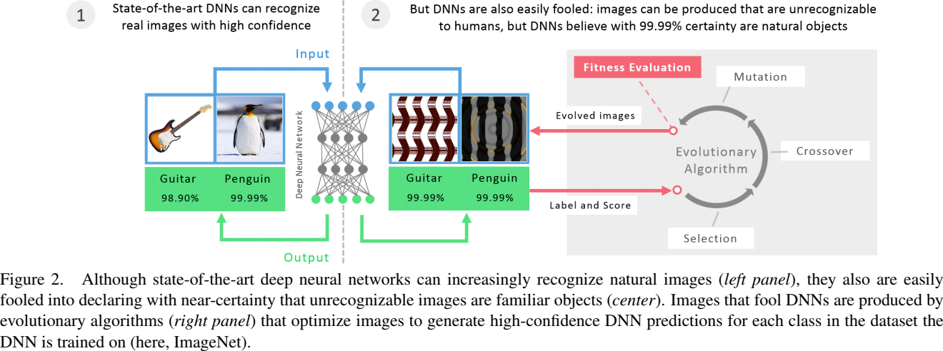] .citation[Nguyen et al, 2014] --- class: middle .center.width-40[<img src="images/part6/fooling.png">] .citation[Nguyen et al, 2014] --- # One pixel attacks .center.width-30[<img src="images/part6/adv-onepx.png">] .citation[Su et al, 2017] --- # Universal adversarial perturbations .center.width-30[<img src="images/part6/universal.png">] .citation[Moosavi-Dezfooli et al, 2016] --- # Fooling deep structured prediction models .center.width-100[] .citation[Cisse et al, 2017] --- class: middle .center.width-70[<img src="images/part6/houdini3.png">] .citation[Cisse et al, 2017] --- # Attacks in the real world .center[<iframe width="640" height="480" src="https://www.youtube.com/embed/YXy6oX1iNoA?&loop=1&start=0" frameborder="0" volume="0" allowfullscreen></iframe> ] --- # Attacks in the real world .center[<iframe width="640" height="480" src="https://www.youtube.com/embed/i1sp4X57TL4&loop=1&start=0" frameborder="0" volume="0" allowfullscreen></iframe> ] --- # Security threat Adversarial attacks pose a **security threat** to machine learning systems deployed in the real world. Examples include: - fooling real classifiers trained by remotely hosted API (e.g., Google), - fooling malware detector networks, - obfuscating speech data, - displaying adversarial examples in the physical world and fool systems that perceive them through a camera. --- class: middle .center.width-90[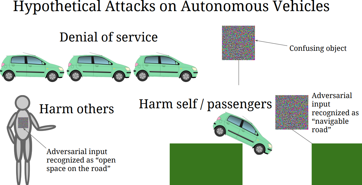] .credit[Credits: [Adversarial Examples and Adversarial Training](https://berkeley-deep-learning.github.io/cs294-dl-f16/slides/2016_10_5_CS294-131.pdf) (Goodfellow, 2016)] --- class: middle # Adversarial defenses --- # Defenses <br> .center.width-80[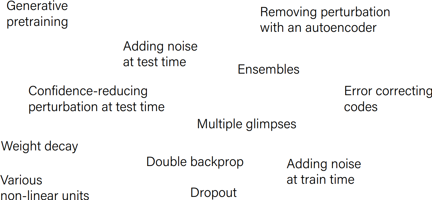] .credit[Credits: [Adversarial Examples and Adversarial Training](https://berkeley-deep-learning.github.io/cs294-dl-f16/slides/2016_10_5_CS294-131.pdf) (Goodfellow, 2016)] --- # Failed defenses <br><br> "In this paper we evaluate ten proposed defenses and demonstrate that none of them are able to withstand a white-box attack. We do this by constructing defense-specific loss functions that we minimize with a strong iterative attack algorithm. With these attacks, on CIFAR an adversary can create imperceptible adversarial examples for each defense. By studying these ten defenses, we have drawn two lessons: existing defenses lack thorough security evaluations, and adversarial examples are much more difficult to detect than previously recognized." .pull-right[(Carlini and Wagner, 2017)] <br><br><br><br><br> .center[Adversarial attacks and defenses remain an **open research problem**.] --- # Recap ## CPU vs GPU ## Visualization of CNN activations and most salient patterns ## Adversarial attacks --- class: end-slide, center count: false The end.