layout: true .center.footer[Marc LELARGE and Andrei BURSUC | Deep Learning Do It Yourself | 14.2 The problems with depth] --- class: center, middle, title-slide count: false ## Going Deeper # 14.2 The problems with depth <br/> <br/> .bold[Andrei Bursuc ] <br/> url: https://dataflowr.github.io/website/ .citation[ With slides from A. Karpathy, F. Fleuret, G. Louppe, C. Ollion, O. Grisel, Y. Avrithis ...] --- class: middle .bigger[Although it was known that _deeper is better_, for decades training deep neural networks was highly challenging and unstable. Besides limited hardware and data there were a few algorithmic flaws that have been fixed/softened in the last decade.] --- # Vanishing gradients Training deep MLPs with many layers has for long (pre-2011) been very difficult due to the **vanishing gradient** problem. - Small gradients slow down, and eventually block, stochastic gradient descent. - This results in a limited capacity of learning. .center.width-60[<img src="images/part14/vanishing-gradient.png">] .caption[Backpropagated gradients normalized histograms (Glorot and Bengio, 2010).<br> Gradients for layers far from the output vanish to zero. ] .citation[X. Glorot and Y. Bengio, Understanding the difficulty of training deep feedforward neural networks; AISTAT 2010] --- Consider a simplified 3-layer MLP, with $x, w\_1, w\_2, w\_3 \in\mathbb{R}$, such that $$f(x; w\_1, w\_2, w\_3) = \sigma\left(w\_3\sigma\left( w\_2 \sigma\left( w\_1 x \right)\right)\right). $$ Under the hood, this would be evaluated as $$\begin{aligned} u\_1 &= w\_1 x \\\\ u\_2 &= \sigma(u\_1) \\\\ u\_3 &= w\_2 u\_2 \\\\ u\_4 &= \sigma(u\_3) \\\\ u\_5 &= w\_3 u\_4 \\\\ \hat{y} &= \sigma(u\_5) \end{aligned}$$ .credit[Credits: G. Louppe, [INFO8010 Deep Learning](https://github.com/glouppe/info8010-deep-learning), ULiège] -- count:false and its derivative $\frac{\text{d}\hat{y}}{\text{d}w\_1}$ as $$\begin{aligned}\frac{\text{d}\hat{y}}{\text{d}w\_1} &= \frac{\partial \hat{y}}{\partial u\_5} \frac{\partial u\_5}{\partial u\_4} \frac{\partial u\_4}{\partial u\_3} \frac{\partial u\_3}{\partial u\_2}\frac{\partial u\_2}{\partial u\_1}\frac{\partial u\_1}{\partial w\_1}\\\\ &= \frac{\partial \sigma(u\_5)}{\partial u\_5} w\_3 \frac{\partial \sigma(u\_3)}{\partial u\_3} w\_2 \frac{\partial \sigma(u\_1)}{\partial u\_1} x \end{aligned}$$ --- class: middle The derivative of the sigmoid activation function $\sigma$ is: .center[<img src="images/part14/activation-grad-sigmoid.png">] $$\frac{\text{d} \sigma}{\text{d} x}(x) = \sigma(x)(1-\sigma(x))$$ Notice that $0 \leq \frac{\text{d} \sigma}{\text{d} x}(x) \leq \frac{1}{4}$ for all $x$. .credit[Credits: G. Louppe, [INFO8010 Deep Learning](https://github.com/glouppe/info8010-deep-learning), ULiège] --- class: middle Assume that weights $w\_1, w\_2, w\_3$ are initialized randomly from a Gaussian with zero-mean and small variance, such that with high probability $-1 \leq w\_i \leq 1$. Then, $$\frac{\text{d}\hat{y}}{\text{d}w\_1} = \underbrace{\frac{\partial \sigma(u\_5)}{\partial u\_5}}\_{\leq \frac{1}{4}} \underbrace{w\_3}\_{\leq 1} \underbrace{\frac{\partial \sigma(u\_3)}{\partial u\_3}}\_{\leq \frac{1}{4}} \underbrace{w\_2}\_{\leq 1} \underbrace{\frac{\sigma(u\_1)}{\partial u\_1}}\_{\leq \frac{1}{4}} x$$ This implies that the gradient $\frac{\text{d}\hat{y}}{\text{d}w\_1}$ **exponentially** shrinks to zero as the number of layers in the network increases. Hence the vanishing gradient problem. - In general, bounded activation functions (sigmoid, tanh, etc) are prone to the vanishing gradient problem. - Note the importance of a proper initialization scheme. .credit[Credits: G. Louppe, [INFO8010 Deep Learning](https://github.com/glouppe/info8010-deep-learning), ULiège] --- # Rectified linear units Instead of the sigmoid activation function, modern neural networks are for most based on **rectified linear units** (ReLU) (Glorot et al, 2011): $$\text{ReLU}(x) = \max(0, x)$$ .center[<img src="images/part14/activation-relu.png">] .credit[Credits: G. Louppe, [INFO8010 Deep Learning](https://github.com/glouppe/info8010-deep-learning), ULiège] --- class: middle Note that the derivative of the ReLU function is $$\frac{\text{d}}{\text{d}x} \text{ReLU}(x) = \begin{cases} 0 &\text{if } x \leq 0 \\\\ 1 &\text{otherwise} \end{cases}$$ .center[<img src="images/part14/activation-grad-relu.png">] For $x=0$, the derivative is undefined. In practice, it is set to zero. .credit[Credits: G. Louppe, [INFO8010 Deep Learning](https://github.com/glouppe/info8010-deep-learning), ULiège] --- class: middle Therefore, $$\frac{\text{d}\hat{y}}{\text{d}w\_1} = \underbrace{\frac{\partial \sigma(u\_5)}{\partial u\_5}}\_{= 1} w\_3 \underbrace{\frac{\partial \sigma(u\_3)}{\partial u\_3}}\_{= 1} w\_2 \underbrace{\frac{\partial \sigma(u\_1)}{\partial u\_1}}\_{= 1} x$$ This **solves** the vanishing gradient problem, even for deep networks! (provided proper initialization) Note that: - The ReLU unit dies when its input is negative, which might block gradient descent. - This is actually a useful property to induce *sparsity*. - This issue can also be solved using **leaky** ReLUs, defined as $$\text{LeakyReLU}(x) = \max(\alpha x, x)$$ for a small $\alpha \in \mathbb{R}^+$ (e.g., $\alpha=0.1$). --- class: middle The steeper slope in the loss surface speeds up the training. .center.width-30[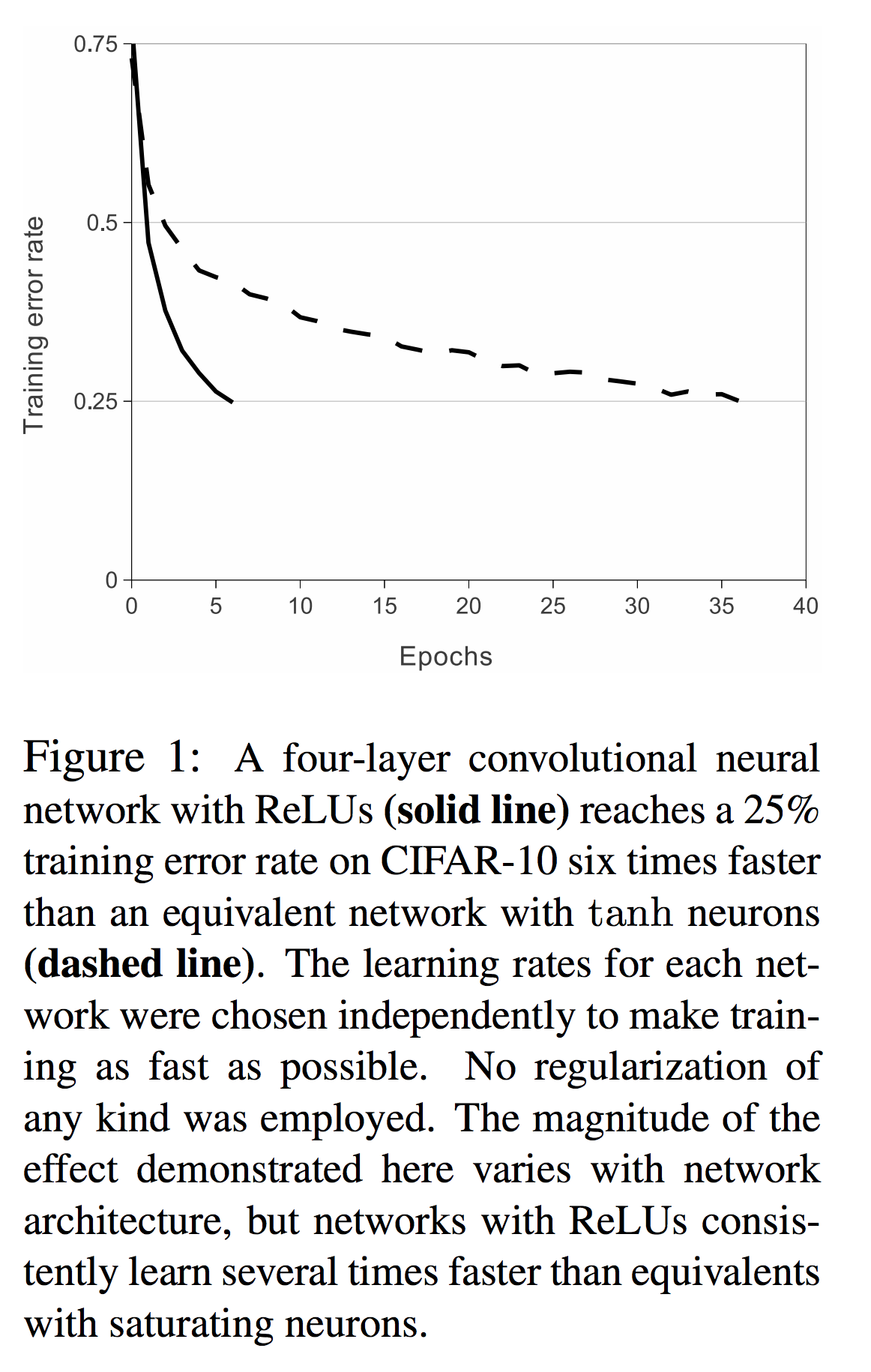] .citation[A. Krizhevsky et al., ImageNet Classification with Deep Convolutional Neural Networks; NIPS 2012] --- # Other activation functions - Several $\text{ReLU}$-like alternatives have been proposed in recent years: $\text{PReLU}$, $\text{ELU}$, $\text{SeLU}$, $\text{SReLU}$ .center.width-50[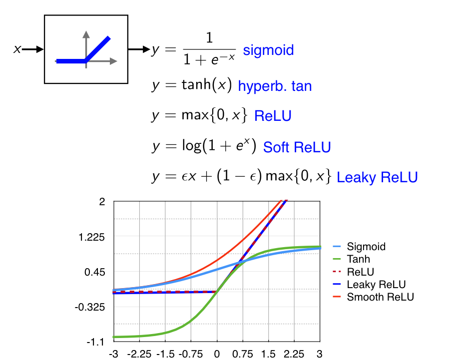] .citation[[Visualising Activation Functions in Neural Networks](https://dashee87.github.io/data%20science/deep%20learning/visualising-activation-functions-in-neural-networks/)] --- class: center, middle # Regularization --- # Under-fitting and over-fitting What if we consider a hypothesis space $\mathcal{F}$ in which candidate functions $f$ are either too "simple" or too "complex" with respect to the true data generating process? .center[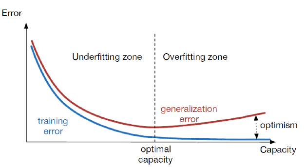] --- class: middle .center.width-40[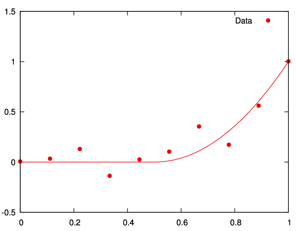] Our goal is to find a function $f$ that makes good predictions on average from given data. We can consider $f$ as a polynomial of degree $D$ defined through its parameters $\mathbf{w} \in \mathbb{R}^D$ such that $$\hat{y} = f(x; \mathbf{w}) = \sum\_{d=0}^D w\_d x^d$$ .credit[Credits: F. Fleuret, [EE-559 Deep Learning](https://fleuret.org/dlc/), EPFL] --- class: middle count: false .center.width-60[] .credit[Credits: F. Fleuret, [EE-559 Deep Learning](https://fleuret.org/dlc/), EPFL] --- class: middle count: false .center.width-60[] .credit[Credits: F. Fleuret, [EE-559 Deep Learning](https://fleuret.org/dlc/), EPFL] --- class: middle count: false .center.width-60[] .credit[Credits: F. Fleuret, [EE-559 Deep Learning](https://fleuret.org/dlc/), EPFL] --- class: middle count: false .center.width-60[] .credit[Credits: F. Fleuret, [EE-559 Deep Learning](https://fleuret.org/dlc/), EPFL] --- class: middle count: false .center.width-60[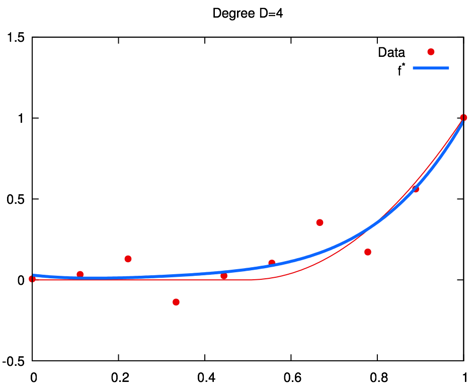] .credit[Credits: F. Fleuret, [EE-559 Deep Learning](https://fleuret.org/dlc/), EPFL] --- class: middle count: false .center.width-60[] .credit[Credits: F. Fleuret, [EE-559 Deep Learning](https://fleuret.org/dlc/), EPFL] --- class: middle count: false .center.width-60[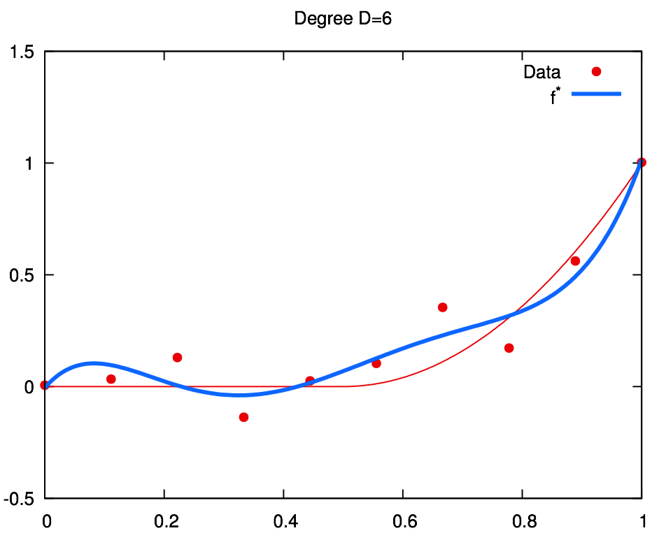] .credit[Credits: F. Fleuret, [EE-559 Deep Learning](https://fleuret.org/dlc/), EPFL] --- class: middle count: false .center.width-60[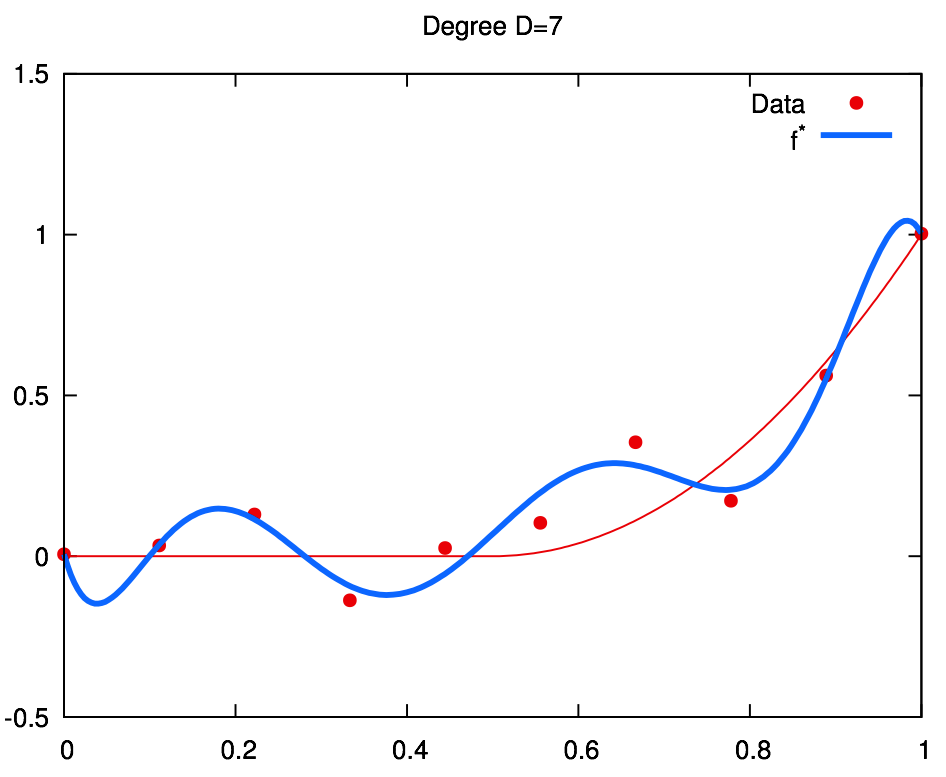] .credit[Credits: F. Fleuret, [EE-559 Deep Learning](https://fleuret.org/dlc/), EPFL] --- class: middle count: false .center.width-60[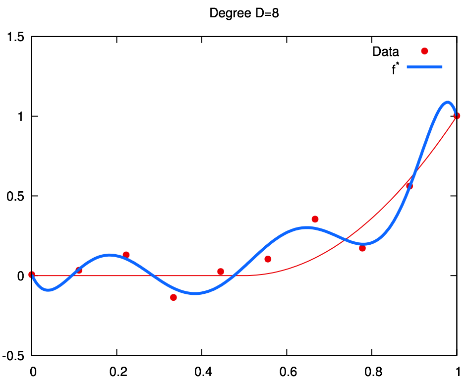] .credit[Credits: F. Fleuret, [EE-559 Deep Learning](https://fleuret.org/dlc/), EPFL] --- class: middle count: false .center.width-60[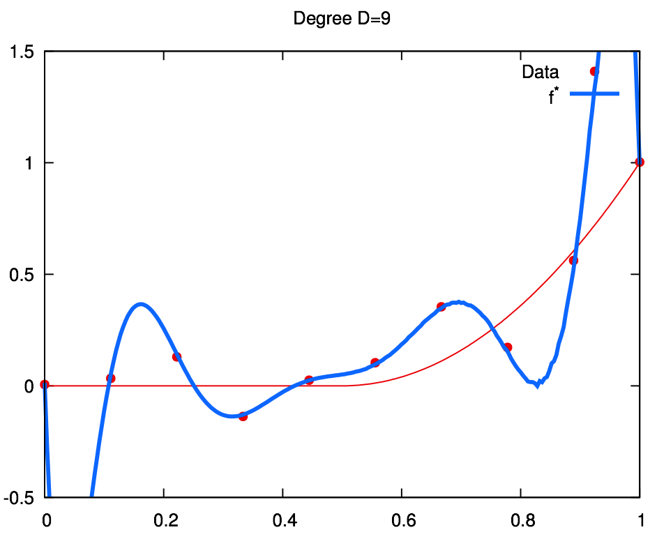] .credit[Credits: F. Fleuret, [EE-559 Deep Learning](https://fleuret.org/dlc/), EPFL] --- class: middle .center.width-60[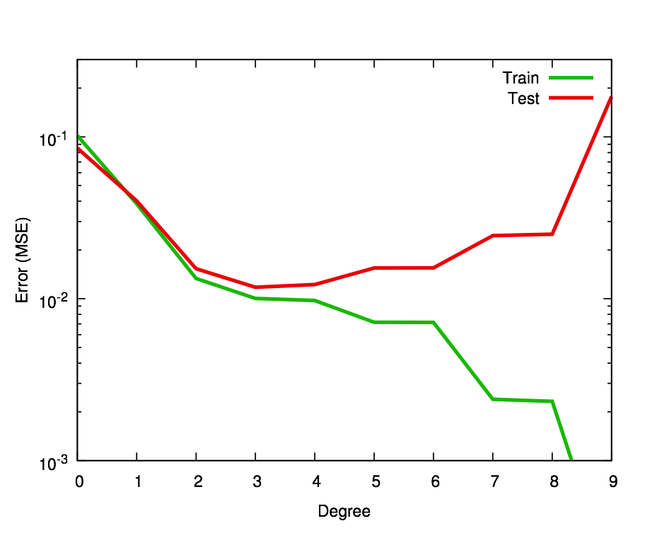] .credit[Credits: F. Fleuret, [EE-559 Deep Learning](https://fleuret.org/dlc/), EPFL] --- class: middle Although it is difficult to define precisely, it is quite clear in practice how to increase or decrease it for a given class of models. For example: - The degree of polynomials; - The number of layers in a neural network; - The number of training iterations; - Regularization terms. --- class: middle # Regularization --- .center.width-100[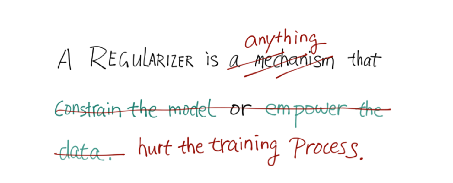] --- # Regularization We can reformulate the previously used squared error loss $$\ell(y, f(x;\mathbf{w})) = (y - f(x;\mathbf{w}))^2$$ to $$\ell(y, f(x;\mathbf{w})) = (y - f(x;\mathbf{w}))^2 + \rho \sum_{d}^{D} w\_d^2$$ <br> .Q.big.center[What will happen now?] --- # Regularization We can reformulate the previously used squared error loss $$\ell(y, f(x;\mathbf{w})) = (y - f(x;\mathbf{w}))^2$$ to $$\ell(y, f(x;\mathbf{w})) = (y - f(x;\mathbf{w}))^2 + \rho \sum_{d}^{D} w\_d^2$$ <br> .center.big[This is called __$L\_2$ regularization__.] --- class: middle .center.width-60[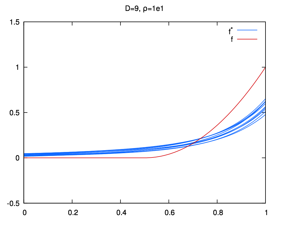] .credit[Credits: F. Fleuret, [EE-559 Deep Learning](https://fleuret.org/dlc/), EPFL] --- class: middle count: false .center.width-60[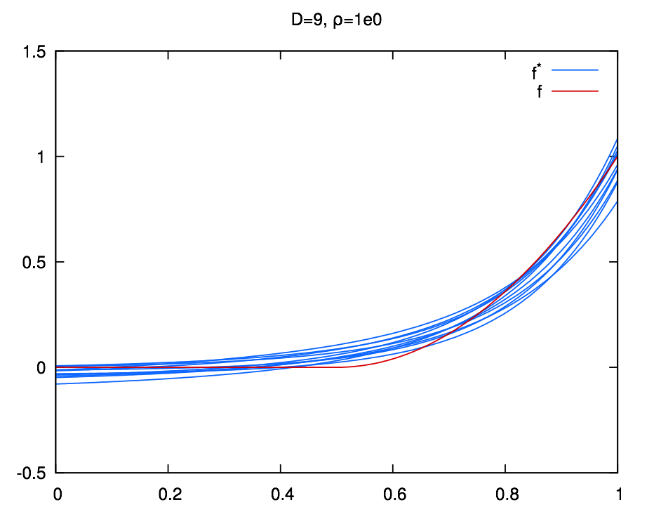] .credit[Credits: F. Fleuret, [EE-559 Deep Learning](https://fleuret.org/dlc/), EPFL] --- class: middle count: false .center.width-60[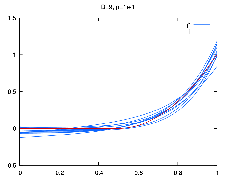] .credit[Credits: F. Fleuret, [EE-559 Deep Learning](https://fleuret.org/dlc/), EPFL] --- class: middle count: false .center.width-60[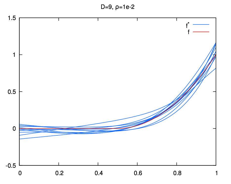] .credit[Credits: F. Fleuret, [EE-559 Deep Learning](https://fleuret.org/dlc/), EPFL] --- class: middle count: false .center.width-60[] .credit[Credits: F. Fleuret, [EE-559 Deep Learning](https://fleuret.org/dlc/), EPFL] --- class: middle count: false .center.width-60[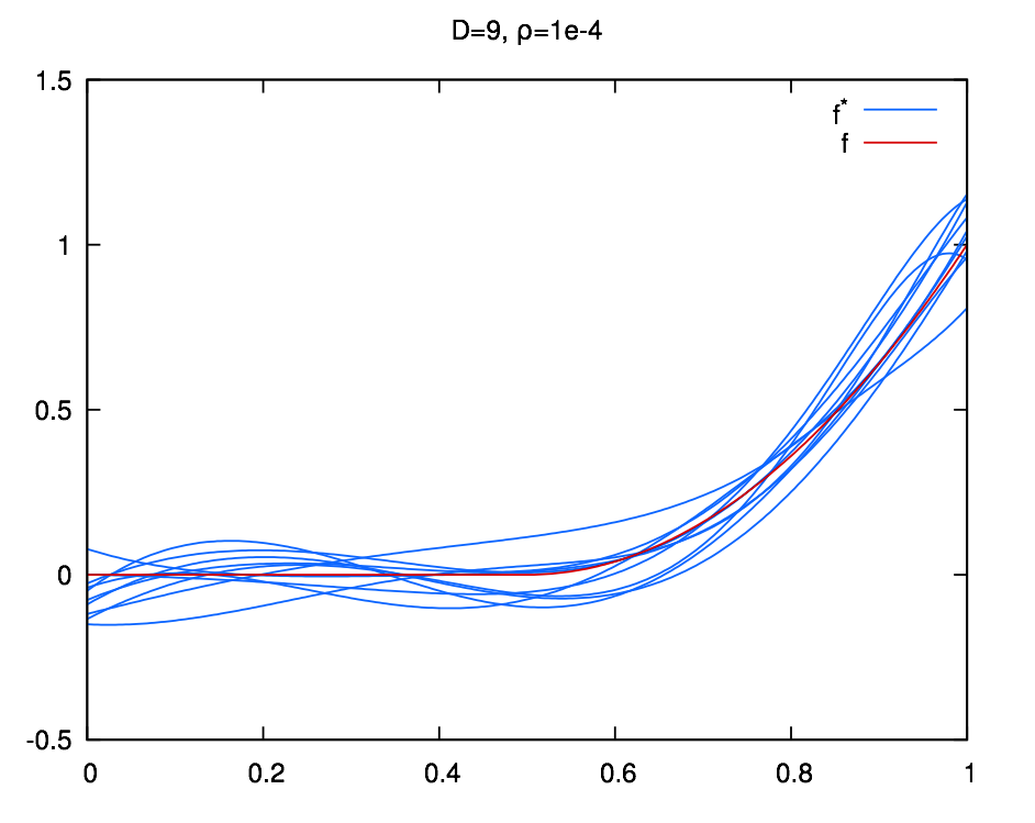] .credit[Credits: F. Fleuret, [EE-559 Deep Learning](https://fleuret.org/dlc/), EPFL] --- class: middle count: false .center.width-60[] .credit[Credits: F. Fleuret, [EE-559 Deep Learning](https://fleuret.org/dlc/), EPFL] --- class: middle count: false .center.width-60[] .credit[Credits: F. Fleuret, [EE-559 Deep Learning](https://fleuret.org/dlc/), EPFL] --- class: middle count: false .center.width-60[] .credit[Credits: F. Fleuret, [EE-559 Deep Learning](https://fleuret.org/dlc/), EPFL] --- class: middle count: false .center.width-60[] .credit[Credits: F. Fleuret, [EE-559 Deep Learning](https://fleuret.org/dlc/), EPFL] --- class: middle count: false .center.width-60[] .credit[Credits: F. Fleuret, [EE-559 Deep Learning](https://fleuret.org/dlc/), EPFL] --- class: middle count: false .center.width-60[] .credit[Credits: F. Fleuret, [EE-559 Deep Learning](https://fleuret.org/dlc/), EPFL] --- class: middle count: false .center.width-60[] .credit[Credits: F. Fleuret, [EE-559 Deep Learning](https://fleuret.org/dlc/), EPFL] --- class: middle count: false .center.width-60[] .credit[Credits: F. Fleuret, [EE-559 Deep Learning](https://fleuret.org/dlc/), EPFL] --- class: middle count: false .center.width-60[] .credit[Credits: F. Fleuret, [EE-559 Deep Learning](https://fleuret.org/dlc/), EPFL] --- class: middle count: false .center.width-60[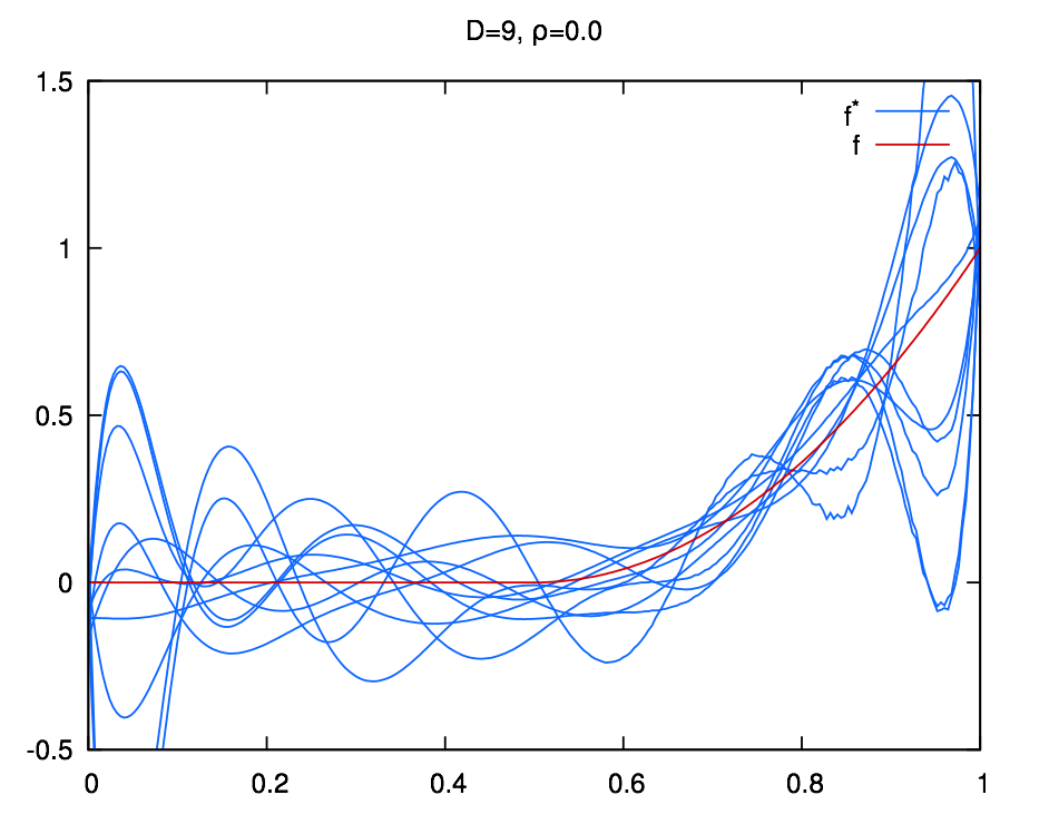] .credit[Credits: F. Fleuret, [EE-559 Deep Learning](https://fleuret.org/dlc/), EPFL] --- class: middle count: false .center.width-60[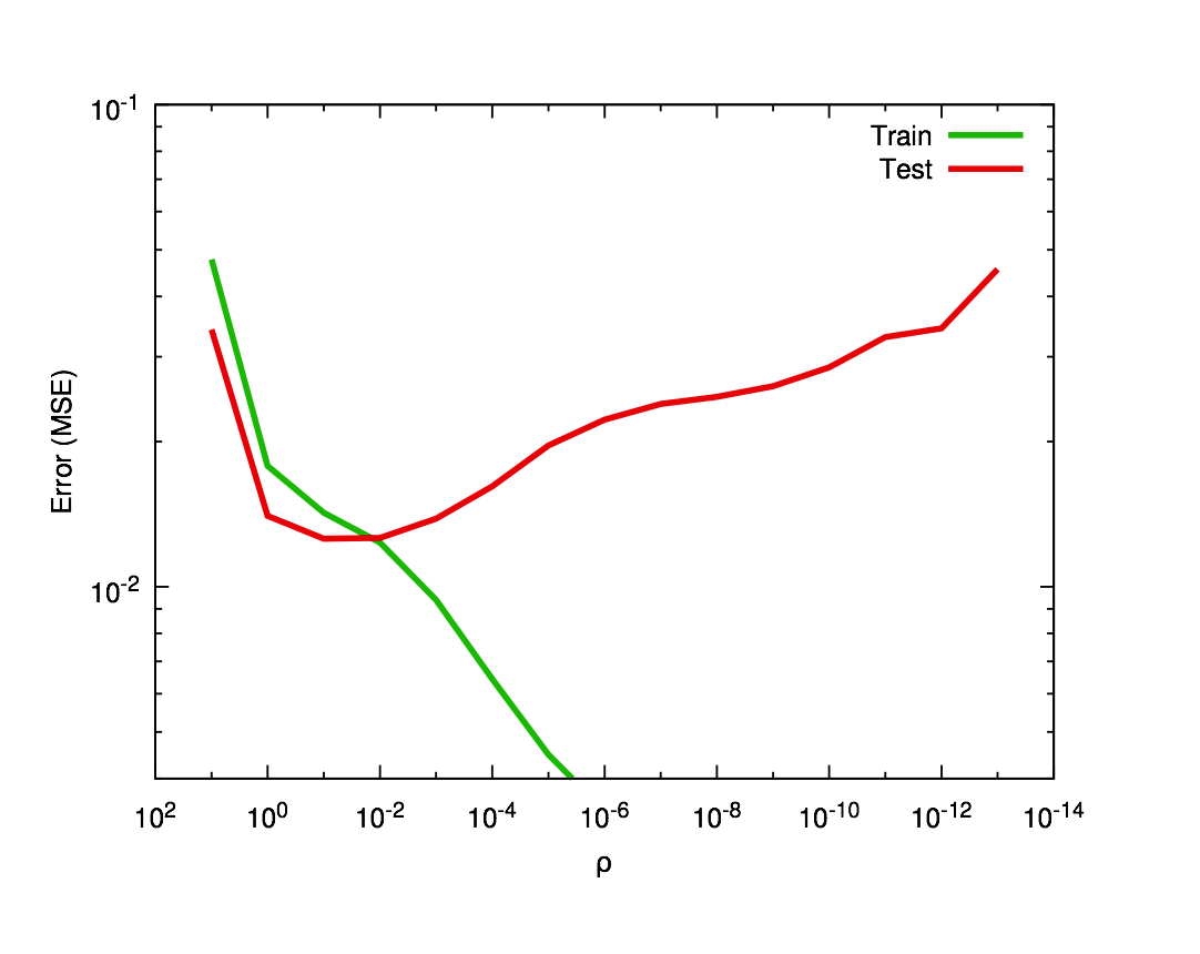] .credit[Credits: F. Fleuret, [EE-559 Deep Learning](https://fleuret.org/dlc/), EPFL] --- # $L\_2$ regularization - in Deep Learning it is ofter referred to as __weight decay__ ```py torch.optim.SGD(params, lr=<required parameter>, momentum=0, dampening=0, weight_decay=0, nesterov=False) ``` ```py torch.optim.Adam(params, lr=0.001, betas=(0.9, 0.999), eps=1e-08, weight_decay=0, amsgrad=False) ``` --- class: middle, center .bigger[So far we have explored generic regularization methods. In the following we will learn deep learning specific regularization strategies.] --- class: end-slide, center count: false The end.