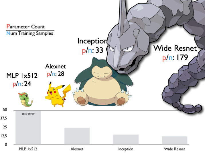
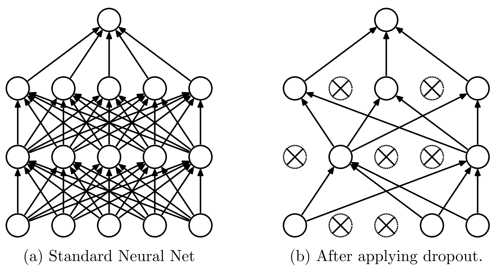
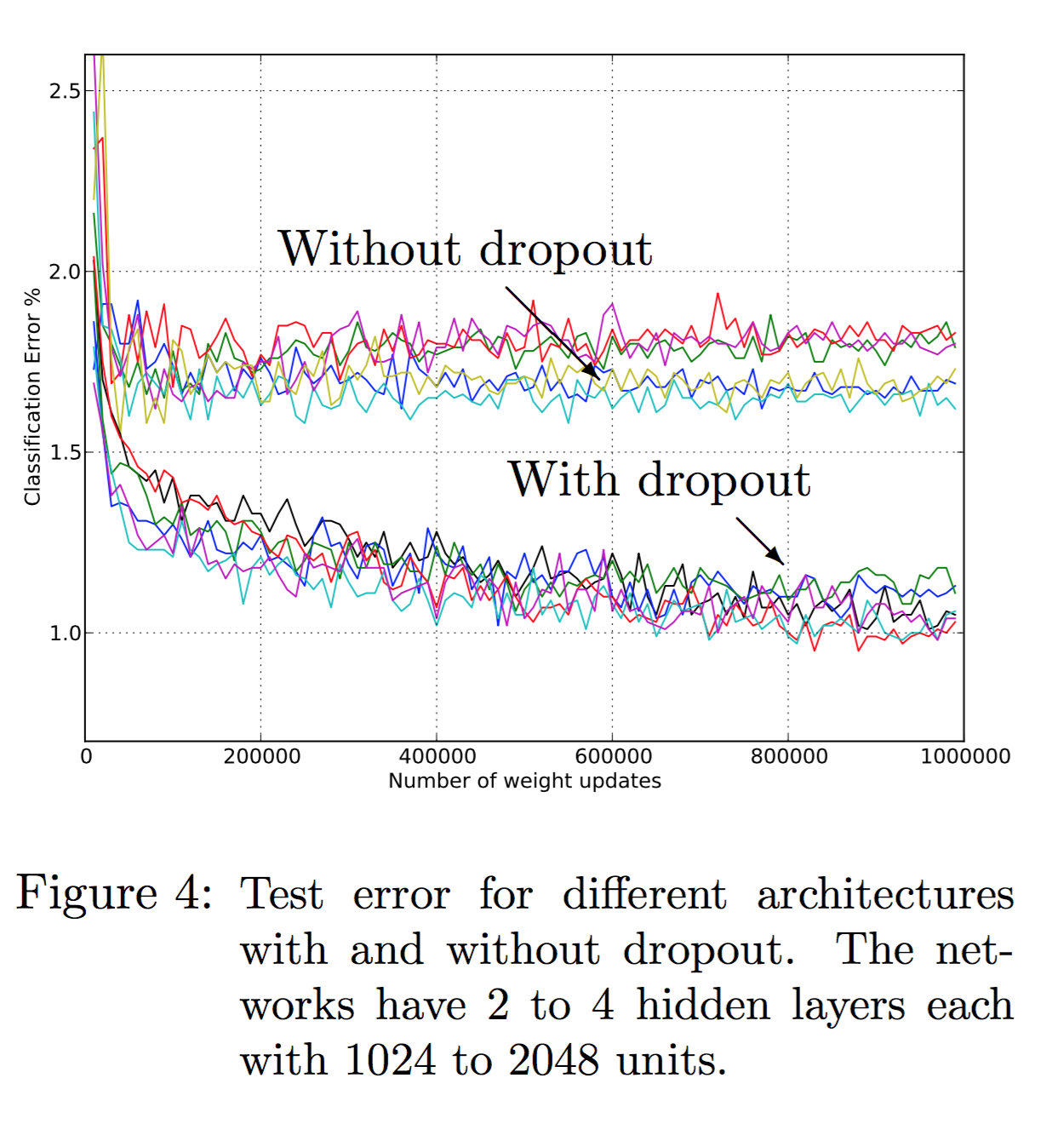
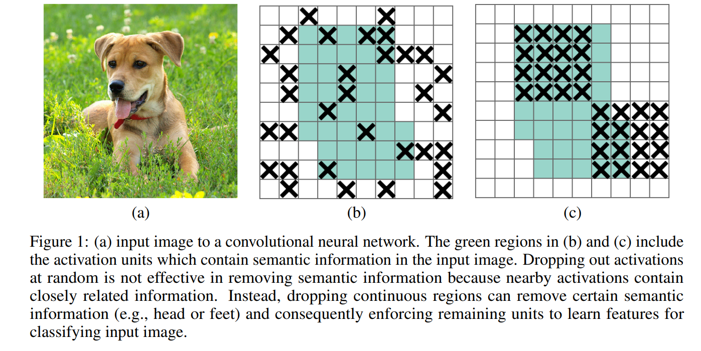
layout: true .center.footer[Marc LELARGE and Andrei BURSUC | Deep Learning Do It Yourself | 15.1 Dropout] --- class: center, middle, title-slide count: false ## Going Deeper # 15.1 Dropout <br/> <br/> .bold[Andrei Bursuc ] <br/> url: https://dataflowr.github.io/website/ .citation[ With slides from A. Karpathy, F. Fleuret, G. Louppe, C. Ollion, O. Grisel, Y. Avrithis ...] --- class: center, middle # Deep regularization --- class: middle .center.width-65[] .citation[C. Zhang et al., Understanding deep learning requires rethinking generalization, ICLR 2017] --- class: middle, center ### Most of the weights of the network are grouped in the final layers. .center.width-80[] --- # VGG-16 .center[ <img src="images/part14/vgg.png" style="width: 600px;" /> ] .citation[K. Simonyan and A. Zisserman, Very deep convolutional networks for large-scale image recognition, NIPS 2014] --- # Memory and Parameters ```md Activation maps Parameters INPUT: [224x224x3] = 150K 0 CONV3-64: [224x224x64] = 3.2M (3x3x3)x64 = 1,728 CONV3-64: [224x224x64] = 3.2M (3x3x64)x64 = 36,864 POOL2: [112x112x64] = 800K 0 CONV3-128: [112x112x128] = 1.6M (3x3x64)x128 = 73,728 CONV3-128: [112x112x128] = 1.6M (3x3x128)x128 = 147,456 POOL2: [56x56x128] = 400K 0 CONV3-256: [56x56x256] = 800K (3x3x128)x256 = 294,912 CONV3-256: [56x56x256] = 800K (3x3x256)x256 = 589,824 CONV3-256: [56x56x256] = 800K (3x3x256)x256 = 589,824 POOL2: [28x28x256] = 200K 0 CONV3-512: [28x28x512] = 400K (3x3x256)x512 = 1,179,648 CONV3-512: [28x28x512] = 400K (3x3x512)x512 = 2,359,296 CONV3-512: [28x28x512] = 400K (3x3x512)x512 = 2,359,296 POOL2: [14x14x512] = 100K 0 CONV3-512: [14x14x512] = 100K (3x3x512)x512 = 2,359,296 CONV3-512: [14x14x512] = 100K (3x3x512)x512 = 2,359,296 CONV3-512: [14x14x512] = 100K (3x3x512)x512 = 2,359,296 POOL2: [7x7x512] = 25K 0 FC: [1x1x4096] = 4096 7x7x512x4096 = 102,760,448 FC: [1x1x4096] = 4096 4096x4096 = 16,777,216 FC: [1x1x1000] = 1000 4096x1000 = 4,096,000 TOTAL activations: 24M x 4 bytes ~= 93MB / image (x2 for backward) TOTAL parameters: 138M x 4 bytes ~= 552MB (x2 for plain SGD, x4 for Adam) ``` .credit[Credits: O. Grisel & C. Ollion, [M2DS Deep Learning](https://m2dsupsdlclass.github.io/lectures-labs/), IP Paris] --- # Memory and Parameters ```md Activation maps Parameters INPUT: [224x224x3] = 150K 0 *CONV3-64: [224x224x64] = 3.2M (3x3x3)x64 = 1,728 *CONV3-64: [224x224x64] = 3.2M (3x3x64)x64 = 36,864 POOL2: [112x112x64] = 800K 0 CONV3-128: [112x112x128] = 1.6M (3x3x64)x128 = 73,728 CONV3-128: [112x112x128] = 1.6M (3x3x128)x128 = 147,456 POOL2: [56x56x128] = 400K 0 CONV3-256: [56x56x256] = 800K (3x3x128)x256 = 294,912 CONV3-256: [56x56x256] = 800K (3x3x256)x256 = 589,824 CONV3-256: [56x56x256] = 800K (3x3x256)x256 = 589,824 POOL2: [28x28x256] = 200K 0 CONV3-512: [28x28x512] = 400K (3x3x256)x512 = 1,179,648 CONV3-512: [28x28x512] = 400K (3x3x512)x512 = 2,359,296 CONV3-512: [28x28x512] = 400K (3x3x512)x512 = 2,359,296 POOL2: [14x14x512] = 100K 0 CONV3-512: [14x14x512] = 100K (3x3x512)x512 = 2,359,296 CONV3-512: [14x14x512] = 100K (3x3x512)x512 = 2,359,296 CONV3-512: [14x14x512] = 100K (3x3x512)x512 = 2,359,296 POOL2: [7x7x512] = 25K 0 *FC: [1x1x4096] = 4096 7x7x512x4096 = 102,760,448 FC: [1x1x4096] = 4096 4096x4096 = 16,777,216 FC: [1x1x1000] = 1000 4096x1000 = 4,096,000 TOTAL activations: 24M x 4 bytes ~= 93MB / image (x2 for backward) TOTAL parameters: 138M x 4 bytes ~= 552MB (x2 for plain SGD, x4 for Adam) ``` .credit[Credits: O. Grisel & C. Ollion, [M2DS Deep Learning](https://m2dsupsdlclass.github.io/lectures-labs/), IP Paris] --- class: middle, center # Dropout --- # Dropout - First "deep" regularization technique - Remove units at random during the forward pass on each sample - Put them all back during test .center.width-60[] .citation[Srivastava et al., Dropout: A Simple Way to Prevent Neural Networks from Overfitting, JMLR 2014] --- # Dropout ## Interpretation - Reduces the network dependency to individual neurons and distributes representation - More redundant representation of data ## Ensemble interpretation - Equivalent to training a large ensemble of shared-parameters, binary-masked models - Each model is only trained on a single data point - __A network with dropout can be interpreted as an ensemble of $2^N$ models with heavy weight sharing__ (Goodfellow et al., 2013) --- # Dropout .center.width-55[] - One has to decide on which units/layers to use dropout, and with what probability $p$ units are dropped. - During training, for each sample, as many Bernoulli variables as units are sampled independently to select units to remove. - To keep the means of the inputs to layers unchanged, the initial version of dropout was multiplying activations by $p$ during test. - The standard variant is the "inverted dropout": multiply activations by $\frac{1}{1-p}$ during training and keep the network untouched during test. --- # Dropout Overfitting noise .center.width-55[] .credit[Credits: O. Grisel & C. Ollion, [M2DS Deep Learning](https://m2dsupsdlclass.github.io/lectures-labs/), IP Paris] --- count: false # Dropout A bit of Dropout .center.width-55[] .credit[Credits: O. Grisel & C. Ollion, [M2DS Deep Learning](https://m2dsupsdlclass.github.io/lectures-labs/), IP Paris] --- count: false # Dropout Too much: underfitting .center.width-55[] .credit[Credits: O. Grisel & C. Ollion, [M2DS Deep Learning](https://m2dsupsdlclass.github.io/lectures-labs/), IP Paris] --- count: false # Dropout .center.width-40[] .citation[Srivastava et al., Dropout: A Simple Way to Prevent Neural Networks from Overfitting, JMLR 2014] --- # Dropout ```py >>> x = torch.full((3, 5), 1.0).requires_grad_() >>> x tensor([[ 1., 1., 1., 1., 1.], [ 1., 1., 1., 1., 1.], [ 1., 1., 1., 1., 1.]]) >>> dropout = nn.Dropout(p = 0.75) >>> y = dropout(x) >>> y tensor([[ 0., 0., 4., 0., 4.], [ 0., 4., 4., 4., 0.], [ 0., 0., 4., 0., 0.]]) >>> l = y.norm(2, 1).sum() >>> l.backward() >>> x.grad tensor([[ 0.0000, 0.0000, 2.8284, 0.0000, 2.8284] [ 0.0000, 2.3094, 2.3094, 2.3094, 0.0000] [ 0.0000, 0.0000, 4.0000, 0.0000, 0.0000]]) ``` --- count: false # Dropout ```py >>> x = torch.full((3, 5), 1.0).requires_grad_() >>> x tensor([[ 1., 1., 1., 1., 1.], [ 1., 1., 1., 1., 1.], [ 1., 1., 1., 1., 1.]]) >>> dropout = nn.Dropout(p = 0.75) >>> y = dropout(x) *>>> y *tensor([[ 0., 0., 4., 0., 4.], * [ 0., 4., 4., 4., 0.], * [ 0., 0., 4., 0., 0.]]) >>> l = y.norm(2, 1).sum() >>> l.backward() >>> x.grad tensor([[ 0.0000, 0.0000, 2.8284, 0.0000, 2.8284] [ 0.0000, 2.3094, 2.3094, 2.3094, 0.0000] [ 0.0000, 0.0000, 4.0000, 0.0000, 0.0000]]) ``` --- # Dropout For a given network ```py model = nn.Sequential(nn.Linear(10, 100), nn.ReLU(), nn.Linear(100, 50), nn.ReLU(), nn.Linear(50, 2)); ``` -- count: false we can simply add dropout layers ```py model = nn.Sequential(nn.Linear(10, 100), nn.ReLU(), * nn.Dropout(), nn.Linear(100, 50), nn.ReLU(), * nn.Dropout(), nn.Linear(50, 2)); ``` --- # Dropout A model using dropout has to be set in __train__ or __test__ mode --- count: false # Dropout A model using dropout has to be set in __train__ or __test__ mode The method `nn.Module.train(mode)` recursively sets the flag `training` to all sub-modules. ```py >>> dropout = nn.Dropout() >>> model = nn.Sequential(nn.Linear(3, 10), dropout, nn.Linear(10, 3)) >>> dropout.training True >>> model.train(False) Sequential ( (0): Linear (3 -> 10) (1): Dropout (p = 0.5) (2): Linear (10 -> 3) ) >>> dropout.training False ``` --- # Dropout A model using dropout has to be set in __train__ or __test__ mode ```py >>> dropout = nn.Dropout() >>> model = nn.Sequential(nn.Linear(3, 10), dropout, nn.Linear(10, 3)) >>> x = torch.full((1, 3), 1.0) *>>> model.train() Sequential ( (0): Linear (3 -> 10) (1): Dropout (p = 0.5) (2): Linear (10 -> 3) ) >>> model(x) *tensor([[ 0.5360, -0.5225, -0.5129]], grad_fn=<ThAddmmBackward>) >>> model(x) *tensor([[ 0.6134, -0.6130, -0.5161]], grad_fn=<ThAddmmBackward>) ``` --- count: false # Dropout A model using dropout has to be set in __train__ or __test__ mode ```py >>> dropout = nn.Dropout() >>> model = nn.Sequential(nn.Linear(3, 10), dropout, nn.Linear(10, 3)) >>> x = torch.full((1, 3), 1.0) >>> model.train() Sequential ( (0): Linear (3 -> 10) (1): Dropout (p = 0.5) (2): Linear (10 -> 3) ) >>> model(x) tensor([[ 0.5360, -0.5225, -0.5129]], grad_fn=<ThAddmmBackward>) >>> model(x) tensor([[ 0.6134, -0.6130, -0.5161]], grad_fn=<ThAddmmBackward>) >>> *>>> model.eval() Sequential ( (0): Linear (3 -> 10) (1): Dropout (p = 0.5) (2): Linear (10 -> 3) ) >>> model(x) *tensor([[ 0.5772, -0.0944, -0.1168]], grad_fn=<ThAddmmBackward>) >>> model(x) *tensor([[ 0.5772, -0.0944, -0.1168]], grad_fn=<ThAddmmBackward>) ``` --- # Spatial Dropout .grid[ .kol-6-12[ - The original Dropout is less compatible with convolutional layers. - Units in a 2d activation map are generally locally correlated, and dropout has virtually no effect. - An alternative is to drop channels instead of individual units. ] .kol-6-12[ ] ] --- count: false # Spatial Dropout .grid[ .kol-6-12[ - The original Dropout is less compatible with convolutional layers. - Units in a 2d activation map are generally locally correlated, and dropout has virtually no effect. - An alternative is to drop channels instead of individual units. ] .kol-6-12[ ```py >>> dropout2d = nn.Dropout2d() >>> x = Variable(Tensor(2, 3, 2, 2).fill_(1.0)) >>> dropout2d(x) Variable containing: (0 ,0 ,.,.) = 0 0 0 0 (0 ,1 ,.,.) = 0 0 0 0 (0 ,2 ,.,.) = 2 2 2 2 (1 ,0 ,.,.) = 2 2 2 2 (1 ,1 ,.,.) = 0 0 0 0 (1 ,2 ,.,.) = 2 2 2 2 [torch.FloatTensor of size 2x3x2x2] ``` ] ] --- #DropBlock .center.width-70[] .center[Masking out continous regions in feature maps] .citation[G. Ghiasi et al.,DropBlock: A regularization method for convolutional networks, NIPS 2018] --- # Gaussian Dropout - we can generalize Bernoulli sampling over neurons, to sampling from other distributions - mutliplying activations and feature maps by a random variable drawn from $\mathcal{N}(1,1)$ works just as well, or perhaps bettern than using Bernoulli noise - this new form of dropout amounts to adding a Gaussian distributed random variable with zero mean and standard deviation equal to the activation of the unit - each hidden activation $h\_i$ is perturbed to: .center[$h\_i+h\_i r$ where $r \sim \mathcal{N}(0,1)$] or .center[$h\_i r'$ where $r' \sim \mathcal{N}(1,1)$] - we can generalize this to $r' \sim \mathcal{N}(1,\sigma^2)$, where $\sigma$ becomes and additional hyperparameter to tune, just like $p$ in standard Bernoulli dropout .citation[Srivastava et al., Dropout: A Simple Way to Prevent Neural Networks from Overfitting, JMLR 2014] --- class: end-slide, center count: false The end.